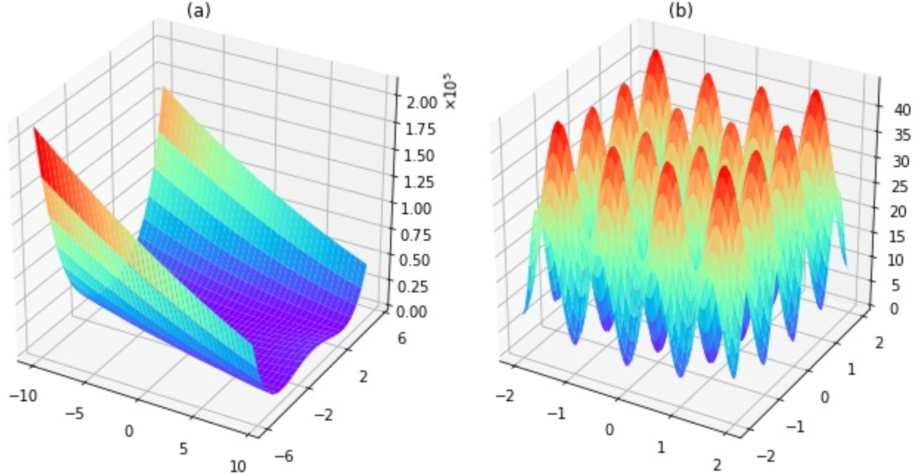
Fig. 1: Plots of black-box functions.
From: Bayesian optimization with adaptive surrogate models for automated experimental design

a The valley of a two-dimensional Rosenbrock function which has the formula \({{{\bf{y}}}}=100{({{{{\bf{x}}}}}_{2}-{x}_{1}^{2})}^{2}+{({{{{\bf{x}}}}}_{1}-1)}^{2}\). b The frequent and regularly distributed local minima of a two-dimensional Rastrigin function which has the formula \({{{\bf{y}}}}=20+\mathop{\sum }\nolimits_{i = 1}^{2}[{{{{\bf{x}}}}}_{i}^{2}-10\cos (2\pi {{{{\bf{x}}}}}_{i})]\).
