Stochastic 3D reconstruction of cracked polycrystalline NMC particles using 2D SEM data

Abstract

Li-ion battery performance is strongly influenced by the 3D microstructure of its cathode particles. Cracks within these particles develop during calendaring and cycling, reducing connectivity but increasing reactive surface, making their impact on battery performance complex. Understanding these contradictory effects requires a quantitative link between particle morphology and battery performance. However, informative 3D imaging techniques are time-consuming, costly and rarely available, such that analyses often have to rely on 2D image data. This paper presents a novel stereological approach for generating virtual 3D cathode particles exhibiting crack networks that are statistically equivalent to those observed in 2D sections of experimentally measured particles. Consequently, 2D image data suffices for deriving a full 3D characterization of cracked cathodes particles. Such virtually generated 3D particles could serve as geometry input for spatially resolved electro-chemo-mechanical simulations to enhance our understanding of structure-property relationships of cathodes in Li-ion batteries.

Introduction

Li-ion batteries are vital to modern technology and transportation^1,2. Current research initiatives in Li-ion technology aim to increase battery energy density while simultaneously extending cycle-life^3,4. To that end, high-voltage LiNi_xMn_yCo_zO₂ (NMCxyz) cathodes are increasingly integrated into energy-dense cells due to their high average voltages (≈3.7 V vs. Li) and high theoretical specific capacities (185–278 mAh g⁻¹)^5,6,7,8,9. Additionally, when cycled within appropriate voltage windows (≤4.3 V vs. Li), these cathodes can reach upwards of a thousand cycles with high capacity retention³. Currently, NMC chemistries are the primary candidates for cathode materials that lead to energy-dense Li-ion batteries, spanning both liquid^{10,11,12,13,14} and solid-state^{15,16,17,18,19} electrolyte systems. However, NMC cathodes can exhibit capacity-fade mechanisms including transition-metal dissolution^20,21, surface reconstruction^8,10, electrolyte reactivity and gassing^8,22,23, and particle cracking^24,25. These fade mechanisms are highly coupled^{9,12,15,26,27,28,29,30}. For example, in liquid systems, particle cracking can expose uncoated active material to liquid electrolyte, resulting in increased electrochemical side reactions and surface reconstruction^8,27. In solid systems, cathode cracking can result in reduced surface area to either the solid-state electrolyte or the electron-conducting phase, resulting in increased charge transfer and ohmic resistance, respectively^17,18,19.

Because a significant amount of cathode capacity-fade mechanisms are related to secondary-particle cracking, researchers typically evaluate cathode “ageing” through qualitative crack analysis^12,28. Cathode particle cracking can occur for different reasons. First, during manufacturing, cathode cracking can occur during the calendaring process^7,31,32. The cracks formed during calendaring typically originate at particle/particle or particle/current-collector contacts and tend to form long cracks that cleave particles. Second, cathode cracking can occur during formation cycles due to non-ideal primary particle grain orientations. These initial “break-in” cracks tend to be small and are significantly influenced by the grain shapes, sizes, and orientations^33,34. Break-in cracking is currently the primary focus for physics-based chemo-mechanical models^{33,35,36,37,38}. Finally, cracks can form during operation when the cathodes are cycled at higher voltage ranges, either due to increased voltage bounds or due to voltage slippage^12,39. At high voltages or during high delithiation demands, the lithium concentration on the cathode surface can drop below a minimum concentration threshold, causing irreversible reconstruction of the host crystal. This reconstruction reduces the specific capacity and induces significant local stain, leading to secondary-particle cracking^29,33.

Currently, structural post-mortem analysis of cathode particle fracture is primarily conducted using 2D scanning electron microscope (SEM) images and X-ray techniques^{11,12,29,40,41,42}. Since a quantitative analysis of such 2D images can be difficult, the comparison of differently aged post-mortem cathodes is often performed by means of visual inspection^11,12,30. Such a qualitative analysis is typically accompanied by quantitative electrochemical analysis (e.g., electrochemical impedance spectroscopy, incremental capacity analysis^12,29) and post-mortem, atomistic-scale surface-sensitive techniques^{11,20,29,42,43}. However, relying on qualitative cracking-extent assessments introduces subjectivity in the analysis, highlighting the need for more quantitative and reproducible methods to characterize cathode-particle fracture. A quantitative analysis of cracks in 2D SEM data has been conducted, e.g., in ref. ^40,41. However, 2D images of cracked particles depict only planar sections of the actual 3D microstructure. In other words, a 2D slice of a cathode electrode represents just a small portion of the 3D system, which includes out-of-plane features, such as tortuous crack connections.

In contrast to 2D crack analysis, it is significantly more difficult to segment and identify crack structures in 3D images^44,45 and to reassemble fragments of fractured particles⁴⁶. This increased difficulty is due to the fact that 3D imaging (e.g., via nano-CT) is often accompanied with a lower resolution than 2D microscopy techniques (e.g., SEM), which produce image data on a similar length scale—i.e., fine structures caused by cracks often exhibit a bad contrast in 3D image data. Moreover, a quantitative crack analysis requires computation of metrics to describe cracks in 3D⁴⁷. Unfortunately, the necessary 3D imaging equipment is expensive and often less available than comparable 2D imaging equipment and their analysis tools^20,48,49. A potential remedy is provided by stochastic 3D modeling, which can generate countless virtual NMC particles exhibiting statistically similar properties as the relatively low number of particles that have been imaged in 3D⁵⁰. In general, realizations of stochastic 3D models for material microstructures, such as those proposed in ref. ^51,52, can serve as geometry inputs for mechanical and electrochemical simulations. These simulations can help to investigate properties like crack propagation in materials and their elastostatic or -plastic responses^33,53,54,55. By performing such simulation studies on generated morphologies quantitative structure-property relationships can be derived^56,57.

As mentioned above, measured 3D image data is not always accessible. Therefore, approaches have been developed to calibrate stochastic 3D models utilizing only 2D image data⁵⁸. Recently, a stochastic nanostructure model based on generative adversarial networks was introduced, which mimics the 3D polycrystalline grain architecture of non-cracked NMC particles⁵⁹ by only using 2D electron backscatter diffraction (EBSD) cross sections for calibration. In the present paper, a stochastic 3D model is proposed that can generate realistic cracks in virtual polycrystalline NMC particles, which propagate along grain boundaries. Similar to the approach considered in ref. ⁶⁰, our model is based on random tessellations, where certain facets are dilated to mimic cracks. In this work, a facet between two grains is either intact or fully cracked without an intermediate case (that is, all surface elements of the facet are either intact or cracked. The model is calibrated and validated by comparing planar cross sections of the stochastic 3D crack network model with 2D SEM image data, utilizing several geometric descriptors characterizing the morphology of the crack phases. Additionally, to emphasize the strength of our stereological modeling approach, geometric descriptors related to effective battery properties are determined, which cannot be reliably derived from 2D images.

Results

The focus of the sections “Electrode materials and cycling history” and “Decomposition of the set of segmented particles into two subsets” is to describe the materials considered in the present paper, as well as the processing of 2D SEM image data of these materials. First, the cathode materials and their cycling history are discussed in section “Electrode materials and cycling history”. Then, in section “Preprocessing and analysis of 2D SEM image data” several image processing techniques are described, where gray-scale images of planar cross sections of the cathodes, obtained by SEM imaging, are phasewise segmented using a 2D U-net and, afterwards, particlewise segmented utilizing a marker-based watershed transform. Additionally, morphological operations are used to denoise the crack phase. Finally, in section “Decomposition of the set of segmented particles into two subsets” the set of segmented 2D images is decomposed into two subsets, based on the predominance of short or long cracks. Later on, the introduced crack model was calibrated to both subsets, to reproduce the wide structural variability of cracked NMC particles.

In sections “Stochastic 3D model for pristine polycristalline NMC particles” and “Extended crack network model”, a stochastic 3D model is proposed, which generates cracks in (simulated) pristine NMC particles hierarchically on different length scales. In section “Stochastic 3D model for pristine polycristalline NMC particles” the tessellation-based model introduced in ref. ⁵⁰ is used to generate pristine polycristalline NMC particles in 3D. Afterwards, in section “Graph representation of pristine grain architectures” an alternative representation of polycristalline architectures is introduced that facilitates modeling of inter-granular cracks. Subsequently, in sections “Single crack model” and “Extended crack network model” crack models for single cracks, crack networks and extended crack networks are proposed.

The calibration of the extended crack network model is pointed out in sections “Minimization problem” and “Model validation.” First, in section “Minimization problem”, we formulate a minimization problem to determine optimal values of model parameters. For this, three different geometric descriptors of image data are utilized, which are introduced in detail in section “Geometric descriptors of 2D image data for model calibration”. These geometric descriptors are used to define a loss function, which measures the discrepancy between experimentally imaged particle cross sections and those drawn from the crack network model. Subsequently, in section “Numerical solution of the minimization problem”, a numerical method is described for solving this minimization problem. Finally, the calibration of the extended crack network model to experimental image data is validated in section “Model validation”.

Electrode materials and cycling history

The active electrode material used in the present paper consisted of LiNi_0.5Mn_0.3Co_0.2O₂ (NMC532) and was taken from the same batch of cells cycled in our previous work⁴¹, where the particles had similar polycrystalline architectures as those shown in ref. ⁶¹. The electrodes consisted of 90 wt% NMC532, 5wt% Timcal C45 carbon and 5wt% Solvay 5130 PVDF binder. The coating thickness was 62 μm with 26.1% porosity.

The cell was formed by charging to 1.5 V, holding at open-circuit for 12 h, and then cycling three times between 3 and 4.1 V using a protocol consisting of C/2 constant-current and constant-voltage at 4.1 V until the current dropped below C/10. The cells were then degassed, resealed, and prepared for fast charging at 20 °C. Subsequently, the cells were cycled using a protocol of fast charging at 6 °C constant current between 3 and 4.1 V followed by constant-voltage hold until 10 min total charge time had elapsed. Charge was followed by 15 min of open circuit and discharge at C/2 to 3 V, followed by a final rest for 15 min. The materials used in this paper were cycled 200 times under these conditions.

Preprocessing and analysis of 2D SEM image data

The NMC electrode material was removed from the cells, and a small sample was cut from the electrode sheet. The sample was then cross-sectioned using an Ar-ion beam cross-sectional polisher (JOEL CP19520). The cross-sectioned face was then imaged in an SEM system with a pixel size of 38.5 nm. A representative cross-section, derived by SEM imaging, is presented in Fig. 1a.

Fig. 1: 2D SEM image data and its segmentation.

2D SEM image (a) and its phasewise segmentation (b), where each pixel is classified as background (white), solid (gray), or crack (black). Note that truncated and small particles with a large eccentricity have been removed.

For image processing, we first describe the image processing steps which were performed in ref. ⁴¹ to segment the 2D SEM image data of the cross sections with respect to phases and particles, i.e., each pixel is classified either as solid phase, crack phase or background, where each particle is assigned with a unique label. Note that the raw image data depicted scale bars for indicating the corresponding length scales (which have been produced by the microscope’s software). Since the scale bars can adversely impact subsequent image processing steps, the inpainting_biharmonic method of the scikit-image package in Python⁶² has been utilized to remove scale bars. Then, a generative adversarial network⁶³ has been deployed to increase the resolution (super-resolution) such that pixel sizes of 14.29 nm have been achieved, facilitating the assignment of pixels to phases (i.e., solid phase, crack phase, and background).

To obtain a phasewise segmentation, a 2D U-net was deployed to classify the phase affiliation for each pixel in 2D SEM cross sections. More precisely, the network’s output is given by pixel-wise probabilities of phase membership. By deploying thresholding techniques onto these pixel-wise probabilities, a phase-wise segmentation has been obtained, see ref. ⁴¹ for further details. In particular, Fig. 1 indicates that the data has been segmented reasonably well, i.e., only a low, statistically negligible number of particles (see bottom left) exhibit larger misclassified areas.

The particle-wise segmentation was obtained by means of a marker-based watershed transform on the Euclidean distance transform, denoted by D in the following. More precisely, $D:W\to {{\mathbb{R}}}_{+}=[0,\infty )$ is a mapping, which assigns each pixel x $\in$ W its distance to the background phase. Here, $W\subset {{\mathbb{Z}}}_{\rho }^{2}$ represents the sampling window, where ${{\mathbb{Z}}}_{\rho }=\{\ldots ,-\rho ,0,\rho ,\ldots \}$ and ρ > 0 denotes the pixel length. Note that the watershed function of the Python package scikit-image⁶² was deployed on − D, where the markers (i.e., the positions of particles to be segmented) are obtained by thresholding D at some distance level r > 0, where r is set equal to 50 pixels. After the application of the watershed algorithm, truncated particles were removed in order to avoid edge effects. In addition, we removed regions within the segmented image that may have resulted from oversegmentation or falsely segmented phases, which can occur due to shine-through effects during SEM imaging. To identify such regions, we first used the GaussianMixture method from the scikit-learn package in Python⁶⁴. This method was employed to fit a mixed bivariate Gaussian distribution (with two components) to the pairs of area-equivalent diameters and eccentricity values of the segmented regions in the image⁶². Note that the eccentricity of a segmented region is defined as the eccentricity of a fitted ellipse that has the same first and second moments. After fitting the mixed Gaussian distribution, its first component, i.e., a bivariate Gaussian distribution, exhibited a mean value vector comprising a relatively large area-equivalent diameter and low eccentricity (which corresponds to circular regions). We assumed that this component corresponds to correctly segmented particles in the image. In contrast, the second component, characterized by a mean vector with smaller area-equivalent diameters and higher eccentricity, was assumed to represent incorrect segmentations. Consequently, we removed regions from the segmentations for which the vector of area-equivalent diameter and eccentricity was more likely to belong to the second component, as determined by the fitted Gaussian mixture model.

Note that a few particles affected by shine-trough effects from SEM imaging remain. However, their small proportion has a negligible impact on the overall statistical properties of the particle set. This procedure is performed on 13 SEM cross sections, each consisting of 5973 × 3079 pixels with a resolution of ρ = 14.29 nm, which corresponds to approximately 85 μm × 44 μm. Note that these 13 cross sections are derived from the same cathode and are partly overlapping. In each cross section, between 43 and 60 particles were detected. An exemplary phasewise segmented cross section is shown in Fig. 1b).

In addition to the preprocessing procedure explained above and proposed in ref. ⁴¹, the following data processing steps have been carried out. First, since some SEM images depict overlapping areas, duplicates were removed. More precisely, all pairs of particles from overlapping images were registered, i.e., for each pair of particles a rigid transformation is determined which maximizes the correspondence of the first particle after application of the transformation with the second particle, where the agreement is measured by means of the cross correlation in scikit-image⁶². If pairs of registered particles exhibit a large correspondence, a duplicate is detected, which is omitted in further analysis. Furthermore, to reduce the number of very small cracks, e.g., caused by noise or by several connected components of the crack phase that actually belong to the same crack, morphological opening, followed by morphological closing, was performed on the crack phase. For both morphological operations, a disk-shaped structuring element with radius r_o = 1 for opening and r_c = 3 for closing was used.

In summary, the image processing procedure described above resulted into 506 images depicting the phasewise segmentation of NMC particles in planar sections, i.e., each pixel is classified either as solid (active NMC material), crack, or background. Each of these images depicts a single cross-section of a NMC particle, which shows a certain network of cracks. In the following sections, an individual particle is denoted by P_ex.

Decomposition of the set of segmented particles into two subsets

In this section, we explain how the set of segmented particles is decomposed into two subsets with predominantly long and short cracks, respectively. This subdivision is motivated by the structural heterogeneity observed in the crack networks of segmented particle cross sections. Later on, the stochastic model is fitted separately to both subsets.

For this classification, for each particle P_ex, we consider a continuous representation in the two-dimensional Euclidean space ${{\mathbb{R}}}^{2}$, denoting its solid phase by ${\Xi}_{\text{solid}}^{\text{(ex)}}\,\subset {{\mathbb{R}}}^{2}$ and its crack phase by ${\Xi}_{\text{crack}}^{\text{(ex)}}\,\subset {{\mathbb{R}}}^{2}$, where each pixel of P_ex is considered as patch (i.e., as a square subset of ${{\mathbb{R}}}^{2}$). Thus, in the following, we will write

$${P}_{{\rm{ex}}}=\left({{{\Xi }}}_{\,{\text{solid}}}^{\text{(ex)}},{{{\Xi}}}_{{\text{crack}}}^{\text{(ex)}}\right)$$

(1)

for the continuous representation of a particle. Furthermore, by ${\mathcal{G}}$ we denote the set of continuous representations of all 506 particles. The dataset ${\mathcal{G}}$ is comprised of particles with sizes ranging from 1.39 to 13.62 μm (in terms of their area-equivalent diameters, denoted by aed(P_ex)).

By visual inspection of segmented particles, it becomes apparent that the crack networks of some particles consist predominantly of short and others of long cracks, see Figs. 1 and 2. Motivated by these morphological differences, the set ${\mathcal{G}}$ is subdivided into two disjoint subsets, ${{\mathcal{G}}}_{{\rm{short}}}$ and ${{\mathcal{G}}}_{{\rm{long}}}$. To decide for a given particle P_ex if it belongs to ${{\mathcal{G}}}_{{\rm{short}}}$ or ${{\mathcal{G}}}_{{\rm{long}}}$, a skeletonization algorithm⁶⁵ was applied to the crack phase of P_ex, where each connected component of the crack phase Ξ_crack is represented by its center line, which we refer to as a skeleton segment. The family of all skeleton segments of a particle P_ex is called skeleton and denoted by ${\mathcal{S}}({P}_{{\rm{ex}}})$.

Fig. 2: Partition of experimentally measured NMC particles.

Segmented NMC particles together with their skeletons (yellow), where the skeleton segment of the longest crack is highlighted in red. The particle on the left-hand side belongs to ${\mathcal{G}}_{\rm{short}}$, consisting of predominantly short cracks, while the particle on the right-hand side belongs to ${{\mathcal{G}}}_{{\rm{long}}}$, exhibiting long cracks.

If the longest crack skeleton segment of a particle P_ex is shorter than or equal to t ⋅ aed(P_ex) for some threshold t > 0, then P_ex is assigned to ${{\mathcal{G}}}_{{\rm{short}}}$, otherwise P_ex is assigned to ${{\mathcal{G}}}_{{\rm{long}}}$ Note that the area-equivalent diameter aed(P) of particle P_ex is given by

$${\text{aed}}({P}_{{\rm{ex}}})=\sqrt{\frac{4\,{\nu }_{2}({{{\Xi}}}_{{\rm{solid}}}\cup \,{{{\Xi }}}_{{\rm{crack}}})}{\pi}},$$

where ν₂(A) denotes the 2-dimensional Lebesgue measure, i.e., the area of a set $A\subset {{\mathbb{R}}}^{2}$. Thus, formally, the sets ${{\mathcal{G}}}_{{\rm{short}}}$ and ${{\mathcal{G}}}_{{\rm{long}}}$ can be written as

$${{\mathcal{G}}}_{{\rm{short}}}=\{{P}_{{\rm{ex}}}\in {\mathcal{G}}:\mathop{\max}\limits_{S\in {\mathcal{S}}({P}_{{\rm{ex}}})}{{\mathcal{H}}}_{1}(S)\le t\cdot \,{\text{aed}}({P}_{{\rm{ex}}})\}\quad \,{\text{and}}\,\quad {{\mathcal{G}}}_{{\rm{long}}}={\mathcal{G}}\setminus {{\mathcal{G}}}_{{\rm{short}}}$$

where ${{\mathcal{H}}}_{1}(S)$ denotes the 1-dimensional Hausdorff measure of a skeleton segment $S\in {\mathcal{S}}({P}_{{\rm{ex}}})$, which corresponds to the length of S. Note that the length of a skeleton segment was approximated by the number of pixels multiplied with the resolution of ρ = 14.29 nm. It turned out that t = 0.55 is a reasonable choice, which splits ${\mathcal{G}}$ into two subsets ${{\mathcal{G}}}_{{\rm{short}}}$ and ${{\mathcal{G}}}_{{\rm{long}}}$, each containing particles from the entire range of observed particle sizes, where ${{\mathcal{G}}}_{{\rm{short}}}$ comprises 423 particles and ${{\mathcal{G}}}_{{\rm{long}}}$ consists of 83 particles. For larger values of t the statistical representativeness of ${{\mathcal{G}}}_{{\rm{long}}}$ diminishes, whereas for smaller values of t we observed that the resulting set ${{\mathcal{G}}}_{{\rm{long}}}$ was comprised of particles with relatively small cracks—which would have made the decomposition of particles into ${{\mathcal{G}}}_{{\rm{short}}}$ and ${{\mathcal{G}}}_{{\rm{long}}}$ redundant.

Stochastic 3D model for pristine polycristalline NMC particles

In ref. ⁵⁰, a spatial stochastic model for the 3D morphology of pristine polycristalline NMC particles has been developed and calibrated by means of tomographic image data. More precisely, nano-CT data depicting the outer shell of NMC particles have been leveraged to calibrate a random field model on the three-dimensional sphere, whose realizations are virtual outer shells of NMC particles that are statistically similar to those observed in the nano-CT data. Furthermore, a random Laguerre tessellation model for the inner grain architecture of NMC particles (which lives on a smaller length scale) has been calibrated using 3D EBSD data.

Note that a Laguerre tessellation in ${{\mathbb{R}}}^{3}$ is a subdivision of the three-dimensional Euclidean space (or some sampling window within ${{\mathbb{R}}}^{3}$) that is given by some marked point pattern $\{({s}_{n},{r}_{n}),n\in {\mathbb{N}}\}$, where ${s}_{n}\in {{\mathbb{R}}}^{3}$ is called a seed or generator point, and ${r}_{n}\in {\mathbb{R}}$ is an (additive) weight, for each $n\in {\mathbb{N}}=\{1,2,\ldots \}$, see refs. ^66,67. The interior of the grain generated by the n-th marked seed point (s_n, r_n) of a Laguerre tessellation is defined as set of points $x\in {{\mathbb{R}}}^{3}$, which are closer to s_n than to all other seed points s_k, k ≠ n, with respect to the “distance function” $d:{{\mathbb{R}}}^{3}\times {{\mathbb{R}}}^{4}\to {\mathbb{R}}$ given by d(x, (s, r)) = ∣x − s∣ − r for all $x,s\in {{\mathbb{R}}}^{3}$ and $r\in {\mathbb{R}}$, where ∣ ⋅ ∣ denotes the Euclidean norm in ${{\mathbb{R}}}^{3}$. Thus, formally, the grain ${g}_{n}\subset {{\mathbb{R}}}^{3}$ generated by the n-th marked seed point (s_n, r_n) is given by

$${g}_{n}=\left\{x\in {{\mathbb{R}}}^{3}\,:\,d(x,({s}_{n},{r}_{n}))\le d(x,({s}_{k},{r}_{k}))\quad \,{\text{for}}\,{\text{all }}\,{k}\,{\ne}\,{n}\right\}.$$

(2)

To compute grains g_n for a given set of marked seed points, we use the GeoStoch library⁶⁸.

Both stochastic models mentioned above, i.e., the random field model for the outer shell and the random tessellation model for the inner grain architecture, have been combined in ref. ⁵⁰, to derive a multi-scale 3D model for pristine NMC particles with full inner grain architecture. Thus, in the first modeling step of the present paper, we will draw realizations from the multi-scale 3D model of ref. ⁵⁰ for the generation of virtual pristine NMC particles, to which cracks will be added in the subsequent modeling steps. Using an analogous notation like that considered in Eq. (1), the simulated pristine NMC particles will be denoted by ${P}_{{\rm{pr}}}=({{{\Xi}}}_{\text{solid}}^{\text{(pr)}},{{\emptyset}})$, where

$$\begin{array}{r}{{{\Xi}}}_{\text{solid}}^{\text{(pr)}}=\mathop{\bigcup}\limits_{{n\in I}}{g}_{n}\subset {{\mathbb{R}}}^{3}\end{array}$$

for some index set $I\subset {\mathbb{N}}$. The stochastic crack model introduced later on assigns facets, i.e., planar grain boundary segments, of the pristine particle P_pr with crack widths to introduce a crack network. To do so, we first derive an alternative graph representation of the Laguerre tessellation {g_n, n $\in$ I} which describes the grain architecture of P_pr.

Graph representation of pristine grain architectures

In the literature, a Laguerre tessellation in ${{\mathbb{R}}}^{3}$ is usually given by a collection of grains ${g}_{n}\subset {{\mathbb{R}}}^{3}$ as defined in Eq. (2). However, alternatively, such a tessellation can be represented as a collection of planar facets given by

$${g}_{n}\cap {g}_{k}=\{x\in {{\mathbb{R}}}^{3}\,:\,d(x,({s}_{n},{r}_{n}))=d(x,({s}_{k},{r}_{k}))\}$$

for $n,k\in {\mathbb{N}}$ with n ≠ k and ${{\mathcal{H}}}_{2}({g}_{n}\cap {g}_{k}) > 0$, where ${{\mathcal{H}}}_{2}({g}_{n}\cap {g}_{k})$ is the 2-dimensional Hausdorff measure of ${g}_{n}\cap {g}_{k}\subset {{\mathbb{R}}}^{3}$, which corresponds to the area of ${g}_{n}\cap {g}_{k}$. Thus, the sets ${g}_{n}\cap {g}_{k}$ are convex plane segments being the intersection of neighboring grains, the union of which is equal to the union of the boundaries ∂g_n of the convex polyhedra g_n considered in Eq. (2).

Furthermore, to describe the neighborhood structure of the facets, we consider the so-called neighboring facet graph, denoted by G = (F, E). The set F of its vertices is the collection of planar facets of the Laguerre tessellation, and E is its set of edges, where two facets $f,{f}^{{\prime} }\in F$ are connected by an edge e $\in$ E if they are adjacent, which means that $f\cap {f}^{{\prime} }$ is a line segment with positive length, i.e., ${{\mathcal{H}}}_{1}(f\cap {f}^{{\prime} }) > 0$, see Fig. 3a, b.

Fig. 3: Workflow to generate cracks.

2D scheme of the workflow to generate an individual crack along grain boundaries. For a (Laguerre) tessellation within a bounded sampling window (a), the neighboring facet graph is determined, i.e., facets are considered to be vertices of the graph (black squares), which are connected by edges (blue) if the underlying facets are adjacent (b). An initial facet (red) is chosen at random and assigned to the set C of crack facets (c). Iteratively, the n-th neighboring facet, which is aligned “best” with the set C is assigned to it (d).

Single crack model

In this section, we describe the stochastic model, which will be used for the insertion of single cracks into virtual NMC particles, whose polycristalline grain architecture is given by a Laguerre tessellation within a certain (bounded) sampling window $W\subset {{\mathbb{R}}}^{3}$, and represented by the neighboring facet graph G = (F, E).

Assuming that cracks propagate along grain boundaries²⁷, we will model cracks as collections of dilated adjacent facets. With regard to the graph-based representation of tessellations, this means that a subset C ⊂ F will be chosen such that for each pair $f,{f}^{{\prime} }\in C$ with $f\,\ne\, {f}^{{\prime}}$, there exists a sequence of adjacent facets f₁, …, f_n $\in$ C such that f₁ = f and ${f}_{n}={f}^{{\prime} }$. This allows generating, if desired, particles with a relatively low quantity of cracked facets, but with relatively long contiguous cracks, which would not be possible with a stochastic approach not consider sequences of adjacent facets.

More precisely, to generate a set of dilated crack facets as described above, an algorithm is proposed consisting of the following steps:

• (i) Initialize the set of crack facets, putting $C={{\emptyset}}$.

• (ii) Generate the number ${n}_{{\rm{facets}}}\in {\mathbb{N}}$ of crack facets, drawing a realization ${\hat{n}}_{{\rm{facets}}} > 0$ from a Weibull distributed random variable N_facets with some scale parameter λ_W > 0 and shape parameter k_W > 0, and putting ${n}_{{\rm{facets}}}={\text{round}}\,({\hat{n}}_{{\rm{facets}}})$, where

  $$\,{\text{round}}\,({\hat{n}}_{{\rm{facets}}})=\left\{\begin{array}{ll}\lfloor {\hat{n}}_{{\rm{facets}}}\rfloor \quad \quad\,{\text{if}}\,\qquad {\hat{n}}_{{\rm{facets}}}-\lfloor {\hat{n}}_{{\rm{facets}}}\rfloor < 0.5,\\ \lfloor {\hat{n}}_{{\rm{facets}}}\rfloor +1\quad\,{\text{else,}}\,\end{array}\right.$$

  (3)

  which means rounding to the closest integer, with $\lfloor {\hat{n}}_{{\rm{facets}}}\rfloor$ denoting the largest integer being smaller than ${\hat{n}}_{{\rm{facets}}}$.

• (iii) Choose an initial facet f $\in$ F at random and assign it to the set of crack facets C. Furthermore, let $g:F\to {{\mathbb{R}}}^{3}$ denote a function, which maps a facet f $\in$ F onto its normal vector v = (v₁, v₂, v₃) with length 1 and v₁ ≥ 0.

• (iv) Compute the average normal vector ${v}_{C}={\sum }_{f\in C}g(f){| {\sum }_{f\in C}g(f)| }^{-1},$ to control the alignment of the next facet, to be assigned to C.

• (v) Determine the set $A=\{f\in F\setminus C:f\cap {f}^{{\prime} }\in E\,{\text{for}} \,{\text{some}}\,{f}^{{\prime} }\in C\}\subset F\setminus C$, containing the facets that are adjacent to C, but not contained in C.

• (vi) Add the facet f $\in$ A given by

  $$f=\mathop{{\rm{argmax}}}\limits_{f\in A}\,| \langle g(f),{v}_{C}\rangle |$$

  (4)

  to C, for which the normal g(f) has the best directional alignment with the average normal vector v_c computed in step (iv), where 〈 ⋅ , ⋅ 〉 denotes the dot product.

• (vii) Repeat steps (iv) to (vi) until #C = n_facets, where # denotes cardinality.

• (viii) Draw a realization δ > 0 from a gamma distributed random variable Δ with some shape parameter $k_{\Delta}$ > 0 and scale parameter $\theta_{\Delta}$ > 0.

• (ix) Dilate each crack facet f $\in$ C using the structuring element ${B}_{\delta }=\{x\in {{\mathbb{R}}}^{3}:| x| \le \delta /2\}$, and determine the set ${\cup}_{f\in {C}}$($f \oplus B_{\delta}$), where ⊕ denotes Minkowski addition. Note that the set ${\cup}_{f\in {C}}$($f \oplus B_{\delta}$) represents a crack where each facet f $\in$ C is dilated with the same thickness δ.

This algorithm is visualized in Fig. 3.

In summary, the stochastic model for single cracks described above is characterized by the 4-dimensional parameter vector ${\theta }_{1}=({\lambda }_{{\rm{W}}},{k}_{{\rm{W}}},{k}_{\Delta },{\theta }_{\Delta })\in {{\mathbb{R}}}_{+}^{4}$, where λ_W and k_W control the length of cracks, whereas $k_{\Delta}$ and $\theta_{\Delta}$ affect their thickness.

Recall the notation ${P}_{{\rm{pr}}}=({{{\Xi}}}_{\text{solid}}^{\text{(pr)}},{{\emptyset}})$ for simulated pristine NMC particles. Analogously, for a given pristine particle ${P}_{{\rm{pr}}}=({{{\Xi}}}_{\text{solid}}^{\text{(pr)}},{{\emptyset}})$, a particle with a single crack will be denoted by ${P}_{{\theta }_{1}}=({{{\Xi}}}_{\text{solid}\,}^{({\theta }_{1})},{{{\Xi }}}_{\text{crack}}^{({\theta }_{1})})$, where ${{{\Xi }}}_{\text{solid}}^{({\theta}_{1})}\cup \,{{{\Xi}}}_{\text{crack}}^{({\theta}_{1})}={{{\Xi }}}_{\text{solid}}^{\text{(pr)}}$, with ${\Xi}_{{\text{solid}}}^{({\theta}_{1})},{\Xi}_{\text{crack}}^{({\theta}_{1})}\subset {{\mathbb{R}}}^{3}$ being the solid and crack phase of ${P}_{{\theta }_{1}}$, respectively. More precisely, it holds that

$$\begin{array}{ll}{{{\Xi}}}_{\text{crack}}^{({\theta}_{1})}=\left\{x\in {{{\Xi }}}_{\text{solid}}^{{\rm{(pr)}}}:{\text{dist}}\,(x,f)\le \frac{\delta}{2}{\text{ for}}\,{\text{some}}\,{f}\in C\right\}\end{array}$$

and ${{{\Xi }}}_{\text{solid}}^{({\theta }_{1})}={{{\Xi }}}_{\text{solid}}^{\text{(pr)}}\setminus {{{\Xi }}}_{\text{crack}}^{({\theta }_{1})}$, where ${\text{dist}}\,(x,f)=\min \{| x-y| :y\in f\}$ denotes the Euclidean distance from $x\in {{\mathbb{R}}}^{3}$ to the set f $\in$ C.

Note that the spatial orientation of the random crack depends solely on the initial facet f, which is chosen at random (uniformly) from the set of facets F. Since the orientation of a facet of a Laguerre tessellation is uniformly distributed on the space of possible facet orientations, the single crack model is isotropic. A potential anisotropy of the crack network could be modeled by modifying the selection criterion formulated in Eq. (4).

Crack network model

Typically, the crack phase of particles observed in experimental 2D SEM data consists of more than one crack and forms complex crack networks, see Fig. 1.

Thus, to model the crack phase of particles consisting of multiple cracks, we draw a realization ${n}_{{\rm{cracks}}}\in {\mathbb{N}}\cup \{0\}$ from a Poisson distributed random variable N_cracks with some parameter λ_P > 0. Furthermore, let ${P}_{{\theta }_{1},1},\ldots ,{P}_{{\theta }_{1},{n}_{{\rm{cracks}}}}$ with ${P}_{{\theta }_{1},i}=({{{\Xi }}}_{\text{solid}}^{({\theta }_{1},i)},{{{\Xi }}}_{\text{crack}}^{({\theta }_{1},i)})$ for i = 1, …, n_cracks denote independent realizations of the single crack model, applied to one and the same pristine particle ${P}_{{\rm{pr}}}=({{{\Xi }}}_{\text{solid}}^{\text{(pr)}},{{\emptyset}})$. Overlaying these realizations results in a realization of the crack network model ${P}_{{\theta }_{2}}=({{{\Xi }}}_{\text{solid}\,}^{({\theta }_{2})},{{{\Xi }}}_{\text{crack}\,}^{({\theta }_{2})})$ with parameter vector

$${\theta }_{2}=({\theta }_{1},{\lambda }_{{\rm{P}}})=({\lambda }_{{\rm{W}}},{k}_{{\rm{W}}},{k}_{\Delta },{\theta }_{\Delta },{\lambda }_{{\rm{P}}})\in {{\mathbb{R}}}_{+}^{5},$$

(5)

where ${{{\Xi }}}_{\text{crack}}^{({\theta }_{2})}=\mathop{\bigcup }\nolimits_{i = 1}^{{n}_{{\rm{cracks}}}}{{{\Xi }}}_{\text{crack}}^{({\theta }_{1},i)}$ and ${{{\Xi }}}_{\text{solid}}^{({\theta }_{2})}={{{\Xi }}}_{\text{solid}}^{\text{(pr)}}\setminus {{{\Xi }}}_{\text{crack}}^{({\theta }_{2})}$.

By visual inspection of the SEM data, see Fig. 1, it is obvious that the distributions of the random number N_cracks and size N_facets of individual cracks should depend on the size of the underlying pristine particle P_pr, i.e., small particles tend to have less and shorter cracks, whereas large particles exhibit more and longer cracks. Therefore, we assume that the scale parameters λ_P, λ_W > 0 considered in Eq. (5) are given by

$${\lambda }_{{\rm{P}}}={\lambda }_{{\rm{P}}}({c}_{{\rm{P}}},{c}_{{\rm{dim}}})={c}_{{\rm{P}}}{\nu }_{3}{\left({{{\Xi }}}_{{\rm{solid}}}^{{\rm{(pr)}}}\right)}^{{c}_{{\rm{dim}}}},\qquad {\lambda }_{{\rm{W}}}={\lambda }_{{\rm{W}}}({c}_{{\rm{W}}},{c}_{{\rm{dim}}})={c}_{{\rm{W}}}{\nu }_{3}{\left({{{\Xi }}}_{{\rm{solid}}}^{{\rm{(pr)}}}\right)}^{1-{c}_{{\rm{dim}}}}$$

(6)

for some constants c_P, c_W > 0, and c_dim $\in$ [0, 1], where ${\nu }_3$ denotes the 3-dimensional Lebesgue measure, i.e., ${\nu }_{3}\left({{{\Xi }}}_{\text{solid}}^{\text{(pr)}}\right)$ is the volume of P_pr. This implies that the porosity

$$p=\frac{{\mathbb{E}}{\nu}_{3}\left({{{\Xi}}}_{\text{crack}}^{({\theta}_{2})}\right)}{{\nu }_{3}\left({{{\Xi}}}_{\text{solid}}^{\text{(pr)}}\right)},$$

of the crack network model ${P}_{{\theta }_{2}}$ does not (or only slightly) depend on the volume ${\nu}_{3}\left({{{\Xi}}}_{\text{solid}}^{\text{(pr)}}\right)$ of the underlying pristine particle P_pr, which can be shown as follows. Since the random variables N_cracks, N_facets, Δ are assumed to be independent, it holds that

$$\begin{array}{rc}p=\frac{{\mathbb{E}}{\nu }_{3}\left({{{\Xi }}}_{\text{crack}}^{({\theta }_{2})}\right)}{{\nu }_{3}\left({{{\Xi }}}_{\text{solid}}^{\text{(pr)}}\right)}&\approx \frac{\alpha {\mathbb{E}}{N}_{{\rm{cracks}}}{\mathbb{E}}{N}_{{\rm{facets}}}{\mathbb{E}}\Delta }{{\nu }_{3}\left({{{\Xi }}}_{\text{solid}}^{{\rm{(pr)}}}\right)}=\frac{\alpha {\lambda }_{{\rm{P}}}{\lambda }_{{\rm{W}}}\,{\gamma }_{{k}_{{\rm{W}}}}{\mathbb{E}}\Delta }{{\nu }_{3}\left({{{\Xi }}}_{\text{solid}}^{\text{(pr)}}\right)},\end{array}$$

(7)

where α > 0 is the mean area of planar facets of the Laguerre tessellation describing the grain architecture of P_pr and ${\gamma }_{{k}_{{\rm{W}}}}=\Gamma (1+\frac{1}{{k}_{{\rm{W}}}})$ with the Gamma function $\Gamma :(0,\infty )\to {{\mathbb{R}}}_{+}$ given by $\Gamma (x)=\mathop{\int}\nolimits_{0}^{\infty }{t}^{z-1}{e}^{-t}\,{\mathrm{d}}t$. Thus, inserting Eq. (6) into Eq. (7), we get that

$$\begin{array}{ll}p\,\approx \frac{\alpha \,{c}_{{\rm{P}}}{\nu }_{3}{\left({{{\Xi }}}_{{\rm{solid}}}^{{\rm{(pr)}}}\right)}^{{c}_{{\rm{dim}}}}\,{c}_{{\rm{W}}}{\nu }_{3}{\left({{{\Xi }}}_{{\rm{solid}}}^{{\rm{(pr)}}}\right)}^{1-{c}_{{\rm{dim}}}}\,{\gamma }_{{k}_{{\rm{W}}}}{\mathbb{E}}\Delta }{{\nu }_{3}\left({{{\Xi }}}_{\text{solid}}^{\text{(pr)}}\right)}\\ \,\qquad={\nu }_{3}\left({{{\Xi }}}_{\text{solid}}^{\text{(pr)}}\right)\,\frac{\alpha \,{c}_{{\rm{P}}}\,{c}_{{\rm{W}}}\,{\gamma }_{{k}_{{\rm{W}}}}{\mathbb{E}}\Delta }{{\nu }_{3}\left({{{\Xi }}}_{\text{solid}}^{\text{(pr)}}\right)}=\,\alpha \,{c}_{{\rm{P}}}\,{c}_{{\rm{W}}}\,{\gamma }_{{k}_{{\rm{W}}}}{\mathbb{E}}\Delta ,\end{array}$$

i.e., the porosity p of the crack network model ${P}_{{\theta }_{2}}$ does not (or only slightly) depend on the volume ${\nu }_{3}\left({{{\Xi }}}_{\,\text{solid}}^{\text{(pr)}\,}\right)$ of the underlying pristine particle P_pr.

Finally, we remark that from now on, utilizing the representation of the scale parameters λ_P and λ_W introduced in Eq. (6), the following modified form of the parameter vector θ₂ of ${P}_{{\theta }_{2}}$ given in Eq. (5) will be used:

$${\theta }_{2}=({c}_{{\rm{W}}},{k}_{{\rm{W}}},{k}_{\Delta },{\theta }_{\Delta },{c}_{{\rm{P}}},{c}_{{\rm{dim}}})\in {{\mathbb{R}}}_{+}^{5}\times [0,1].$$

(8)

Extended crack network model

Recall section “Decomposition of the set of segmented particles into two subsets”, where the set of experimentally measured 2D SEM images ${\mathcal{G}}$ was split into two classes, ${\mathcal{G}}_{\rm{short}}$ and ${\mathcal{G}}_{\rm{long}}$, containing particle cross sections showing either predominantly short or long cracks. Nevertheless, each crack network exhibited on these cross sections, still consists of both, (relatively) short as well as (relatively) long cracks, see Fig. 2.

This is the reason why the crack network model introduced above turned out to be insufficiently flexible. Therefore, we extend this model by realizing it twice on the same pristine particle ${P}_{{\rm{pr}}}=({{{\Xi }}}_{\text{solid}}^{\text{(pr)}},{{\emptyset}})$, with two different parameter vectors

$$\begin{array}{ll}\qquad\quad{\theta }_{2}^{(1)}=\left({c}_{\text{W}}^{(1)},{k}_{{\rm{W}}}^{(1)},{k}_{\Delta }^{(1)},{\theta }_{\Delta }^{(1)},{c}_{{\rm{P}}}^{(1)},{c}_{\text{dim}\,}^{(1)}\right)\\{\text{and}}\,\,\quad{\theta }_{2}^{(2)}=\left({c}_{\,\text{W}}^{(2)},{k}_{{\rm{W}}}^{(2)},{k}_{\Delta }^{(2)},{\theta }_{\Delta }^{(2)},{c}_{{\rm{P}}}^{(2)},{c}_{\text{dim}\,}^{(2)}\right).\end{array}$$

In this way, we obtain two independently cracked particles

$${P}_{{\theta }_{2}^{(1)}}=\left({{{\Xi }}}_{\text{solid}}^{({\theta }_{2}^{(1)})},{{{\Xi }}}_{\text{crack}}^{({\theta }_{2}^{(1)})}\right)\qquad \,{\text{and}}\,\qquad {P}_{{\theta }_{2}^{(2)}}=\left({{{\Xi }}}_{\text{solid}}^{({\theta }_{2}^{(2)})},{{{\Xi }}}_{\text{crack}}^{({\theta }_{2}^{(2)})}\right),$$

which are used to get the extended crack network model ${P}_{\theta }=({{{\Xi }}}_{\text{solid}}^{(\,\theta \,)},{{{\Xi}}}_{\text{crack}}^{(\theta)})$ with $\theta =({\theta }_{2}^{(1)},{\theta }_{2}^{(2)})$, exhibiting a sufficiently large variety of short and long cracks, where

$${{{\Xi }}}_{\text{crack}}^{\text{(}\,\theta \,\text{)}\,}={{{\Xi }}}_{\,\text{crack}\,}^{({\theta }_{2}^{(1)})}\cup {{{\Xi }}}_{\text{crack}}^{({\theta }_{2}^{(2)})}\qquad \,{\text{and}}\,\qquad {{{\Xi }}}_{\text{solid}}^{\text{(}\,\theta \,\text{)}\,}={{{\Xi }}}_{\text{solid}}^{\text{(pr)}}\setminus {{{\Xi }}}_{\text{crack}}^{\text{(}\,\theta \,\text{)}\,}.$$

(9)

By visual inspection of the segmented SEM data, see Fig. 2, it seems clear that short and long cracks exhibit similar thicknesses. This observation motivates a reduction of model parameters by setting ${k}_{\Delta }={k}_{\Delta }^{(1)}={k}_{\Delta }^{(2)}$ and ${\theta }_{\Delta }={\theta }_{\Delta }^{(1)}={\theta }_{\Delta }^{(2)}$. Furthermore, we assume that the influence of the volume ${\nu}_{3}\left({{{\Xi}}}_{\text{solid}}^{\text{(pr)}}\right)$ of the underlying pristine particle P_pr on the distributions of the number and size of cracks is the same for short and long cracks, i.e., we assume that ${c}_{\,\text{dim}}^{(1)}={c}_{{\rm{dim}}}^{(2)}={c}_{{\rm{dim}}}$. Thus, the number of model parameters is reduced from 12 to 9, leading to the parameter vector

$$\theta =\left({c}_{\,\text{W}}^{(1)},{k}_{{\rm{W}}}^{(1)},{c}_{{\rm{P}}}^{(1)},{c}_{{\rm{W}}}^{(2)},{k}_{{\rm{W}}}^{(2)},{c}_{{\rm{P}}}^{(2)},{k}_{\Delta },{\theta }_{\Delta },{c}_{{\rm{dim}}}\right)\in {{\mathbb{R}}}_{+}^{8}\times [0,1]$$

(10)

of the extended crack network model, where ${c}_{\,\text{W}}^{(i)},{k}_{\text{W}\,}^{(i)}$ control the length, ${c}_{\,\text{P}\,}^{(i)}$ the number and $k_{\Delta}$, $\theta_{\Delta}$, the thickness of cracks for i $\in$ {1, 2}, whereas c_dim controls the influence of the volume ${\nu }_{3}\left({{{\Xi }}}_{\text{solid}}^{\text{(pr)}}\right)$ of P_pr on the distributions of the number and size of cracks.

It is important to note that the crack network model as well as the extended crack network model inherit isotropy from the single crack model.

Minimization problem

The extended crack network model parameters are separately fitted to both partitions, ${\mathcal{G}}_{\rm{short}}$ and ${\mathcal{G}}_{\rm{long}}$, of the experimental data set ${\mathcal{G}}$ considered in section “Decomposition of the set of segmented particles into two subsets". Thus, the optimization of the parameter vector θ given in Eq. (10) is performed twice, for ${\mathcal{G}}_{\rm{short}}$ and ${\mathcal{G}}_{\rm{long}}$, where the discrepancy between geometric descriptors of experimental image data and simulated image data drawn from the extended crack network model is minimized. Figs. 4 and 5 illustrate cross section realizations of virtual particles drawn from the extended crack network model fitted to ${\mathcal{G}}_{\rm{short}}$ and ${\mathcal{G}}_{\rm{long}}$, respectively, alongside experimentally imaged cross sections.

Fig. 4: Visual validation: short cracked particles.

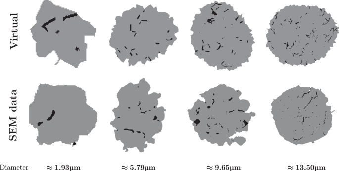
Particle cross sections across various size classes, drawn from the extended crack network model calibrated to ${\mathcal{G}}_{\rm{short}}$ (top row) and corresponding representatives of ${\mathcal{G}}_{\rm{short}}$ (bottom row). The cross sections were scaled to the same size, while their actual sizes are indicated by their area-equivalent diameters.

Fig. 5: Visual validation: Long cracked particles.

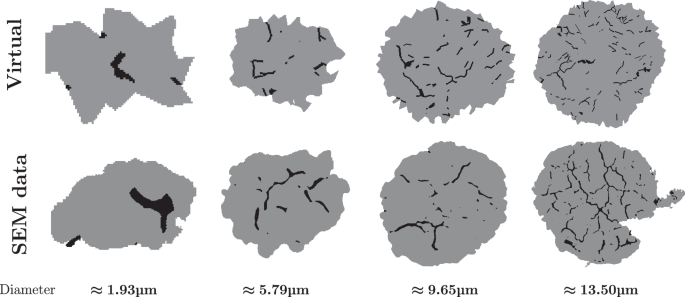
Particle cross sections across various size classes, drawn from the extended crack network model calibrated to ${\mathcal{G}}_{\rm{long}}$ (top row) and corresponding representatives of ${\mathcal{G}}_{\rm{long}}$ (bottom row). The cross sections were scaled to the same size, while their actual sizes are indicated by their area-equivalent diameters.

Furthermore, it is important to note that the crack network morphology may significantly vary across different cross-section sizes, see Fig. 1. To avoid systematic errors arising from comparing experimental and simulated cross sections of different sizes, we introduce several cross-section size classes. Thus, experimental and simulated cross-sections are only compared if they are approximately of the same size. More specifically, a simulated particle cross-section is compared to the average of all experimental cross-sections in the same size class.

For the sake of simplicity, we will use the following abbreviating notation, writing ${\mathcal{G}}$ instead of ${\mathcal{G}}_{\rm{short}}$ and ${\mathcal{G}}_{\rm{long}}$. Furthermore, for each d > 0, let ${\left.{\mathcal{G}}\right\vert }_{d}$ be the restriction of ${\mathcal{G}}$ to all particle cross sections P_ex whose area-equivalent diameter aed(P_ex) belongs to the interval B_ℓ(d) = [jℓ, (j + 1)ℓ) with given length ℓ > 0, where the integer $j\in {\mathbb{N}}\cup \{0\}$ is chosen such that d $\in$ [jℓ, (j + 1)ℓ). It turned out that an interval length of ℓ ≈ 1.29 μm balances a reasonable number of experimental cross sections in each bin and, simultaneously, preserves a sufficiently fine subdivision of the entire dataset ${\mathcal{G}}$, where this subdivision results into 11 size intervals [0, ℓ), …[10ℓ, 11ℓ), with 11ℓ ≈ 14.1 μm. Note that the interval length of ℓ ≈ 1.29 μm corresponds to \approx 90 pixels of the experimental data. However, since the stochastic 3D model for pristine NMC particles, described in section “Stochastic 3D model for pristine polycristalline NMC particles”, has been calibrated to 3D nano-CT data⁵⁰, it happens that for some randomly oriented planes $E\subset {{\mathbb{R}}}^{2}$, the cross sections ${P}_{\theta }\cap E$ of 3D particles drawn from the extended crack network model P_θ are larger than the ones observed in the dataset ${\mathcal{G}}$, which were measured by the 2D SEM technique. Thus, if the area-equivalent diameter of ${P}_{\theta }\cap E$ is larger than 11ℓ, which is the upper bound of the largest size class B_ℓ(10) of the experimental data set ${\mathcal{G}}$ (for both cases ${\mathcal{G}}={{\mathcal{G}}}_{{\rm{short}}}$ and ${\mathcal{G}}={{\mathcal{G}}}_{{\rm{long}}}$), then ${P}_{\theta }\cap E$ is not considered in the minimization procedure.

This leads to the minimization problem

$$\widehat{\theta }=\mathop{{\rm{argmin}}}\limits_{\theta \in {{\mathbb{R}}}_{+}^{8}\times [0,1]}\,{\mathbb{E}}L({P}_{\theta }\cap E,{\left.{\mathcal{G}}\right\vert }_{\text{aed}({P}_{\theta }\cap E)}),$$

(11)

where the expectation in Eq. (11) extends over cross sections ${P}_{\theta }\cap E$ such that aed(${P}_{\theta }\cap E$) ≤ 11ℓ, and L( ⋅ , ⋅ ) is some loss function, which measures the discrepancy between the cross section ${P}_{\theta }\cap E$ of the extended crack network model P_θ and particle cross sections belonging to the restriction ${\left.{\mathcal{G}}\right\vert }_{\text{aed}({P}_{\theta }\cap E)}$ of ${\mathcal{G}}$.

Loss function

We now specify the loss function L( ⋅ , ⋅ ) considered in Eq. (11), utilizing the following geometric particle descriptors: the two-point coverage probabilities prob_crack and prob_solid, the crack-size distribution prob_size and the distance-to-background distribution prob_dist, which are formally introduced in section “Geometric descriptors of 2D image data for model calibration”. Recall that the purpose of the loss function is to measure the discrepancy between experimentally imaged particle cross sections and those drawn from the extended crack network model. In particular, the loss function will be utilized subsequently to solve the minimization problem introduced in Eq. (11).

Let ${\mathcal{G}}$ denote some set of experimentally imaged particle cross sections, e.g., ${\mathcal{G}}={{\mathcal{G}}}_{{\rm{short}}}$. Furthermore, let

$$\begin{array}{r}{\overline{\text{prob}}}_{{\rm{solid}}}({\mathcal{G}})=\frac{1}{\#{\mathcal{G}}}\sum _{P=({{{\Xi }}}_{{\rm{solid}}},{{{\Xi }}}_{{\rm{crack}}})\in {\mathcal{G}}}{\text{prob}}_{{\rm{solid}}}(P).\end{array}$$

be the componentwise average of the vector of relative frequencies given in Eq. (14). The averages ${\overline{\text{prob}}}_{{\rm{crack}}}({\mathcal{G}}),{\overline{\text{prob}}}_{{\rm{size}}}({\mathcal{G}})$ and ${\overline{\text{prob}}}_{{\rm{dist}}}({\mathcal{G}})$ for the two-point coverage probability of the crack phase, crack-size distribution and distance-to-background distribution are defined analogously. The loss function considered in Eq. (11) is then given by

$$\begin{array}{rc}L\left({P}_{\theta }\cap E,{\left.{\mathcal{G}}\right\vert }_{\text{aed}({P}_{\theta })}\right)&=\,{\text{error}}\,\left({\text{prob}}_{{\rm{crack}}}({P}_{\theta }\cap E),{\overline{\text{prob}}}_{{\rm{crack}}}\left({\left.{\mathcal{G}}\right\vert }_{\text{aed}({P}_{\theta }\cap E)}\right)\right)\\ &\,+\,{\text{error}}\,\left({\text{prob}}_{{\rm{solid}}}({P}_{\theta }\cap E),{\overline{\text{prob}}}_{{\rm{solid}}}\left({\left.{\mathcal{G}}\right\vert }_{\text{aed}({P}_{\theta }\cap E)}\right)\right)\\ &\,+\,{\text{error}}\,\left({\text{prob}}_{{\rm{size}}}({P}_{\theta }\cap E),{\overline{\text{prob}}}_{{\rm{size}}}\left({\left.{\mathcal{G}}\right\vert }_{\text{aed}({P}_{\theta }\cap E)}\right)\right)\\ &\,+\,{\text{error}}\,\left({\text{prob}}_{{\rm{dist}}}({P}_{\theta }\cap E),{\overline{\text{prob}}}_{{\rm{dist}}}\left({\left.{\mathcal{G}}\right\vert }_{\text{aed}({P}_{\theta }\cap E)}\right)\right),\end{array}$$

where error( ⋅ , ⋅ ) is an error function which quantifies the discrepancy between a random cross section ${P}_{\theta }\cap E$ of the extended crack network model P_θ, and the set ${\left.{\mathcal{G}}\right\vert }_{\text{aed}}({P}_{\theta }\cap E)$ of experimentally imaged cross sections. More precisely, we consider the truncated mean absolute error

$$\begin{array}{r}\,{\text{error}}\,(x,y)=\frac{1}{{n}_{+}}\mathop{\sum }\limits_{i=1}^{{n}_{+}}| {x}_{i}-{y}_{i}| \end{array}$$

(12)

for $x=({x}_{1},\ldots ,{x}_{n}),y=({y}_{1},\ldots ,{y}_{n})\in {{\mathbb{R}}}^{n}$, where n₊≤n is the smallest integer j $\in$ {1, …, n} such that x_i = y_i = 0 for all i $\in$ {j + 1, …, n}.

Note that truncating the sum in Eq. (12) at n₊≤n is motivated by the fact that the components of the vectors of relative frequencies considered in section “Geometric descriptors of 2D image data for model calibration,” are equal to zero from a certain index. For the two-point coverage probabilities prob_solid( ⋅ ) and prob_crack( ⋅ ) occurring in Eqs. (14) and (15), respectively, this happens when the size of the particle cross section is smaller than h_max ≈ 850 nm. Furthermore, for prob_size( ⋅ ) and prob_dist( ⋅ ), some cross sections may contain only features smaller than a certain threshold. Truncating the sum in Eq. (12) ensures that the sum of absolute values of the right-hand side of Eq. (12) is normalized with the actual number of non-zero components of both vectors $x,y\in {{\mathbb{R}}}^{n}$. Thus, this approach prevents that the error considered in Eq. (12) is not appropriately weighted, which could occur if many components of $x,y\in {{\mathbb{R}}}^{n}$ are equal to zero.

Numerical solution of the minimization problem

For solving the minimization problem stated in Eq. (11), a Nelder-Mead approach⁶⁹ is utilized, where a Monte Carlo simulation technique⁷⁰ is employed in each iteration step of the Nelder-Mead algorithm to approximate the expected value of the loss $L\left({P}_{\theta }\cap E,{\left.{\mathcal{G}}\right\vert }_{\text{aed}}({P}_{\theta })\right)$.

This process involves averaging over numerous cross sections ${P}_{\theta }^{(i)}\cap {E}^{(i)}$, where ${P}_{\theta }^{(i)}$ is a realization of the extended crack network model P_θ, and E⁽ⁱ⁾ is a realization of the randomly orientated plane $E\subset {{\mathbb{R}}}^{3}$ for each i = 1, …, n and some integer $n\in {\mathbb{N}}$. Recall that P_θ is an isotropic model, i.e., the realizations of P_θ exhibit a statistically similar behavior in each direction. Thus, it would be sufficient, to intersect each realization ${P}_{\theta }^{(i)}$ of P_θ with a single plane ${E}_{\text{x},v}\subset {{\mathbb{R}}}^{3}$, where E_x,v denotes a plane that is orthogonal to the x-axis and has a certain distance v > 0 from the origin $o\in {{\mathbb{R}}}^{3}$. However, to keep the computational effort low and, simultaneously, increase the robustness of averaging, each realization ${P}_{\theta }^{(i)}$ is intersected at multiple distances along the x-, y-, and z- axis, respectively. Furthermore, to avoid interpolations of the pixelized image data, cross sections are only taken at integer heights along the coordinate axes.

First, 100 pristine particles are drawn from the stochastic 3D model for polycrystalline NMC particles. Then, in each iteration step of the Nelder-Mead minimization algorithm, 32 out of these 100 particles, denoted by ${P}_{\text{pr}}^{(i)}=({{{\Xi}}}_{\text{solid}}^{(\text{pr}\,,i)},{{\emptyset}})$ for i = 1, …, 32, are chosen with a probability proportional to their volume-equivalent diameter. Note that this selection method corresponds to the probability of intersecting a particle by a randomly chosen plane, as this is done in 2D SEM imaging⁷¹.

Each pristine particle ${P}_{\,\text{pr}\,}^{(i)}$ serves as input for generating a realization of the extended crack network model P_θ, which results in 32 realizations of P_θ, denoted by ${P}_{\theta }^{(i)}=({{{\Xi }}}_{\,\text{solid}\,}^{(\theta ,i)},{{{\Xi }}}_{\,\text{crack}\,}^{(\theta ,i)})$ for I = 1, …, 32. Additionally, for each realization ${P}_{\theta }^{(i)}$, multiple cross sections are generated by intersecting each simulated particle ${P}_{\theta }^{(i)}$ at 10, 20, …, 90% of its size along the x-,y- and z-axis, respectively. This yields 32 realizations of P_θ, each sliced at 9 positions along 3 axes, which finally results into 32 × 9 × 3 = 864 cross sections per iteration step.

More formally, for each simulated particle ${P}_{\theta }^{(i)}$, we assume without loss of generality that it is located in the positive octant ${{\mathbb{R}}}_{+}^{3}={\left[0,\infty \right)}^{3}\subset {{\mathbb{R}}}^{3}$ and touches the xy-plane, xz-plane and yz-plane. Furthermore, let ${\text{diam}}_{{\rm{x}}}({P}_{\theta }^{(i)})$ denote the Feret diameter of ${P}_{\theta }^{(i)}$⁷² along the x-axis, which is given by

$${\text{diam}}_{{\rm{x}}}({P}_{\theta}^{(i)})=\max \left\{v > 0:\left(\mathop{\Xi}\nolimits_{\text{solid}}^{{(\theta ,i)}}\,{\cup}\,\mathop{\Xi}\nolimits_{\text{crack}}^{(\theta ,i)}\right)\cap {E}_{{\text{x}},v}\,\ne\, {{\emptyset}}\right\},$$

(13)

i.e., ${\text{diam}}_{{\rm{x}}}({P}_{\theta }^{(i)})$ describes the size of ${P}_{\theta }^{(i)}$ in x-direction. Analogously, the Feret diameters of ${P}_{\theta }^{(i)}$ along the y- and z- axis will be denoted by ${\text{diam}}_{{\rm{y}}}({P}_{\theta }^{(i)})$ and ${\text{diam}}_{{\rm{z}}}({P}_{\theta }^{(i)})$, where the plane E_x,v on the right-hand side of Eq. (13) is replaced by planes E_y,v and ${E}_{\text{z},v}\in {{\mathbb{R}}}^{3}$ that are orthogonal to the y- and z-axis, respectively, and have the distance v > 0 to the origin.

Then, the expected loss ${\mathbb{E}}L\left({P}_{\theta }\cap E,{\left.{\mathcal{G}}\right\vert }_{\text{aed}({P}_{\theta })}\right)$, occurring in Eq. (11), is numerically approximated by

$${\mathbb{E}}L({P}_{\theta }\cap E,{\left.{\mathcal{G}}\right\vert }_{\text{aed}}({P}_{\theta }\cap E))\approx \frac{1}{864}\mathop{\sum }\limits_{i=1}^{32}\sum _{\text{a}\,\in \{\text{x,y,z}\}}\mathop{\sum }\limits_{j=1}^{9}L\left({P}_{\theta }^{(i)}\cap E({\text{a}}\,,j,{P}_{\theta }^{(i)}),{\left.{\mathcal{G}}\right\vert }_{\text{aed}}\left({P}_{\theta }^{(i)}\cap E(\text{a},j,{P}_{\theta }^{(i)}),\right)\right)$$

where $E(\,{\text{a}},j,P)={E}_{\text{a},\text{round}(j/10\cdot {\text{diam}}_{{\rm{a}}}(P))}$ and round( ⋅ ) denotes rounding to the closest integer, as defined in Eq. (3).

Thus, in summary, to find the optimal parameter vector $\widehat{\theta }$ which solves the minimization problem given in Eq. (11), in each iteration step of the Nelder-Mead algorithm we choose 32 pristine particles out of a pool of 100 realizations of the stochastic 3D model. These selected particles serve as input for the extended crack network model P_θ, where the expected loss is approximated by averaging over 864 cross sections.

Recall that the optimization procedure described above was separately applied to both data sets, ${\mathcal{G}}_{\rm{short}}$ and ${\mathcal{G}}_{\rm{long}}$, resulting in two calibrated models which generate particles exhibiting predominately short or long cracks. In the following, we will refer to the extended crack network model calibrated to ${\mathcal{G}}_{\rm{short}}$ and ${\mathcal{G}}_{\rm{long}}$ as ${P}_{{\hat{\theta }}_{\text{short}}}$ and ${P}_{{\hat{\theta }}_{\rm{long}}}$, where samples drawn from these two models are called short- and long-cracked particles, respectively.

Model validation

To validate the extended crack network model, which has been calibrated to experimental image data, the probability densities of several geometric descriptors, stated in section “Geometric descriptors of 2D image data for model validation” are estimated using particle cross sections of 200 model realizations drawn from each of the extended crack models ${P}_{{\hat{\theta }}_{\rm{short}}}$ and ${P}_{{\hat{\theta }}_{\rm{long}}}$. For a visual impression of realizations of the fitted model, we refer to Fig. 6, which presents clipped 3D renderings of virtually generated cracked NMC particles. To ensure comparability, only 2D cross sections of the 3D realizations have been taken into account, which are extracted, similarly as described in “Numerical solution of the minimization problem”, at 10%, 20%, …, 90% of the particle size along x-,y-, and z-direction, resulting into 9 ⋅ 3 ⋅ 200 = 5400 cross sections for both crack scenarios. For each of these cross sections, the porosity, mean local entropy, number of branching points, as well as the number and length of crack segments are determined. Their probability densities, along with those derived from experimental 2D SEM data, have been computed via kernel density estimation, see Fig. 7.

Fig. 6: 3D renderings of cracked particles.

Exemplary clipped 3D renderings of virtually generated cracked NMC particles, drawn from the extended crack network model. Cracks are indicated in red color, whereas individual grains are visualized in randomly chosen shades of blue. The top row, shows particles drawn from the extended crack model calibrated to ${\mathcal{G}}_{\rm{short}}$, whereas the bottom row corresponds to ${\mathcal{G}}_{\rm{long}}$. The left column features a particle with a volume-equivalent diameter of ≈ 4.6 μm, while the right column shows one of ≈12.5 μm.

Fig. 7: Model validation.

Probability densities of porosity (a), chord lengths (b), mean local entropy (c), number of branching points (d), number (e) and length of crack segments (f). Blue areas indicate densities computed from SEM data, whereas orange areas correspond to densities for planar cross sections of 3D realizations of the extended crack network model. Within each subplot, the left column corresponds to the data set ${\mathcal{G}}_{\rm{short}}$, and the right column to ${\mathcal{G}}_{\rm{long}}$. The horizontal dashed lines indicate the mean values of the respective descriptors.

When comparing the probability densities shown in Fig. 7, derived for each case from simulated and experimental data, respectively, it becomes clearly visible that these pairs of densities exhibit similar shapes, indicating a suitable choice of model type and a quite good fit of model parameters, for both data sets ${\mathcal{G}}_{\rm{short}}$ and ${\mathcal{G}}_{\rm{long}}$. Even in cases where these pairs of probability densities are slightly different from each other, like the densities of the porosity of short-cracked particles (Fig. 7a), left pair of densities), their mean values, represented by horizontal dashed lines, fit very well. On the other hand, for example, the porosity distribution of long-cracked particles (Fig. 7a), the right pair of densities) exhibits a slightly larger deviation of its mean value with respect to the corresponding mean value derived from simulated data. Nevertheless, qualitatively, the overall shapes of the probability densities match quite well in all cases.

In summary, the probability densities derived from simulated and experimentally measured image data show a high degree of agreement, indicating that the crack networks observed in 2D SEM data are accurately represented by the stochastic 3D model.

Discussion

We now deploy the stochastic 3D model ${P}_{\hat{\theta}}$ of cracked particles that has been calibrated by means of 2D data to investigate the transport-relevant descriptors stated in section “Transport-relevant particle descriptors in 3D” for simulated 3D particles drawn from ${P}_{\hat{\theta }}$. In particular, we investigate the probability distributions of the (relative) specific surface area and the mean relative shortest path length (for solid and liquid electrolyte) associated with the stochastic 3D model ${P}_{\hat{\theta}}$. More precisely, we will provide a detailed discussion of the corresponding probability densities of these descriptors, separately for the stochastic 3D model ${P}_{{\hat{\theta }}_{\rm{short}}}$ calibrated to the data set ${\mathcal{G}}_{\rm{short}}$, and for ${P}_{{\hat{\theta }}_{\rm{long}}}$ calibrated to ${\mathcal{G}}_{\rm{long}}$.

First, we draw 200 realizations from ${P}_{{\hat{\theta }}_{\rm{short}}}$ which we denote by P⁽ⁱ⁾ for i = 1, …, 200. By computing the transport-relevant descriptors for these realizations, we obtain four sample data sets, denoted by ${\{{\tau }_{{\rm{LE}}}({P}^{(i)})\}}_{i = 1}^{200},\,{\{{\tau }_{{\rm{SE}}}({P}^{(i)})\}}_{i = 1}^{200},\,{\{\sigma ({P}^{(i)})\}}_{i = 1}^{200}$ and ${\{{\sigma }_{{\rm{rel}}}({P}^{(i)})\}}_{i = 1}^{200}$. Then, by means of kernel density estimation on each of these four sets, we get probability densities of the corresponding transport-relevant particle descriptors, see the blue plots in Figs. 8 and 9. Furthermore, the same procedure was applied to 200 realizations drawn from ${P}_{{\hat{\theta }}_{\rm{long}}}$ to determine probability densities of the particle descriptors, see the green plots in Figs. 8 and 9.

Fig. 8: Mean relative shortest path lengths.

Probability densities of mean relative shortest path lengths τ_LE(P) and τ_SE(P) for liquid (a) and solid electrolyte (b). Each subfigure shows two probability densities, where the green (left) areas correspond to the probability densities computed from short-cracked particles and the blue (right) areas indicate the probability densities derived from long-cracked particles.

Fig. 9: Specific surface area.

Probability densities of the specific surface area σ(P) (a) for pristine particles (purple) and for cracked particles drawn from the stochastic 3D models ${P}_{{\hat{\theta }}_{\rm{short}}}$ (green) and ${P}_{{\hat{\theta }}_{\rm{long}}}$ (blue). Probability densities of the relative specific surface area σ_rel(P) (b) for cracked particles drawn from ${P}_{{\hat{\theta }}_{\rm{short}}}$ (green) and ${P}_{{\hat{\theta }}_{\rm{long}}}$ (blue), respectively.

Note that the transport-relevant particle descriptors, with the exception of the specific surface area σ(P), are computed by comparing descriptors of simulated cracked particles with those of the underlying pristine counterparts. Consequently, for pristine particles the mean relative shortest path length as well as the relative specific surface area are deterministic (i.e., non-random) quantities, being equal to 1. Therefore, when considering probability distributions of relative transport-relevant descriptors, only the specific surface area of pristine particles, see Fig. 9a (purple), is of further interest.

The comparison of the probability densities shown in Figs. 8 and 9 provides us with quantitative insight into the transport behavior of cracked 3D particles, even though initially only 2D data was available. For example, an intuitive result is that shortest path lengths decrease after cracking for liquid electrolyte systems, i.e., the mean relative shortest path lengths are typically smaller than 1, see Fig. 8a. This is to be expected as cracks can be flooded by the liquid electrolyte, leading to shorter transport paths. On the other hand, shortest path lengths increase for solid electrolyte , even though the relative increase is marginal, i.e., only slightly above 1, see Fig. 8b).

These general trends can be observed for both variants of the calibrated stochastic 3D model, ${P}_{{\hat{\theta }}_{\rm{short}}}$ and ${P}_{{\hat{\theta }}_{\rm{long}}}$. However, when comparing both models, we observe that—in the case of liquid electrolyte—mean shortest path lengths seem to decrease more significantly for long-cracked particles rather than for short-cracked ones. For solid electrolyte systems, the difference in mean shortest path lengths between short- and long-cracked particles is much smaller, taking into account the finer length scale of the y-axis on the right-hand side of Fig. 8.

In the case of liquid electrolyte, an explanation for the existence of shorter transport paths is the fact that transport paths, which are originating in the active material phase, have the option to end at the interface between active material and crack phases, instead of ending at the background. In other words, caused by cracking, the set of possible endpoints of transport paths originating in the active material becomes larger, which possibly leads to a decrease of shortest path lengths. On the other hand, in the case of solid electrolyte, only a small fraction of shortest transport paths seems to be affected by cracking (which can cause obstacles to form). Consequently, we observe mean relative shortest path lengths close to 1, see Fig. 8b).

With respect to specific surface area, see Fig. 9a), we observe that both scenarios (i.e., short- and long-cracked particles) lead to an increase of this geometric particle descriptor—an effect that is more pronounced for long-cracked particles generated by ${P}_{{\hat{\theta }}_{\rm{long}}}$. Moreover, the relative specific surface area quantifies this increase compared to the underlying pristine particle. Short-cracked particles exhibit an average increase in their specific surface area by a factor of 1.5 in comparison to their pristine counterparts, whereas this factor is equal to 2 for long-cracked particles, see Fig. 9b.

It is important to note that the transport-relevant particle descriptors discussed in this section, namely the mean relative shortest path length and the relative specific surface area of cracked particles, are just examples of numerous further descriptors of 3D particles, which quantify their morphology, influencing the effective properties of Li-ion batteries. Such descriptors cannot be adequately estimated from 2D cross sections, as they provide only limited information about the complex 3D geometry of cracked NMC particles. In particular, the tortuous nature of cracks cannot be fully captured by 2D cross sections, since it strongly depends on the spatial orientation of the cutting plane.

Thus, the presented stereological approach to stochastic 3D modeling of cracked particles enables the estimation of such structural descriptors from virtual 3D particles, which are statistically consistent with the 2D cross sections used for model calibration. In future studies, the method will be validated by statistically comparing virtually generated 3D particles by the model (that has been calibrated with 2D image data) with experimentally acquired 3D image data of particles. After further validation with 3D image data, the virtually generated 3D NMC particles by our stereological approach will be leveraged to obtain structure-property relationships of cathode materials in Li-ion batteries, by conducting additional (experimentally validated) chemomechanical simulations, where realizations of the presented model will serve as geometry input.

Summing up, this paper presents a novel approach for generating virtual 3D cathode particles with crack networks that are statistically equivalent to those observed in 2D cross-sections of experimentally manufactured particles, where a stochastic 3D model is developed that inserts cracks into virtually generated NMC particles, requiring solely 2D image data for model calibration.

An essential advantage of our model is that it enables the generation and analysis of a large number of virtual particle morphologies in 3D, whose planar 2D sections exhibit similar statistics as planar sections of experimentally manufactured particles. This computer-based procedure is cheaper, faster and more reliable than analyzing just a few experimentally manufactured particles. One reason for this is the circumstance that the acquisition of tomographic image data for a statistically representative number of particles can be expensive in both time and resources.

On the other hand, virtual particles generated by our stochastic 3D model allow for a more rigorous quantification of cracked NMC particles, i.e., by characterizing their 3D morphology and, subsequently, by conducting spatially resolved mechanical and electrochemical simulations examining their structure-properties relationships. This supports the analysis and comparison of different cycling conditions such as varying C-rate, operating temperature, or number of cycles.

It is important to emphasize that the stochastic model presented in this paper for the 3D morphology of cracked NMC particles is characterized by a small number of (nine) interpretable parameters. In contrast to convolutional neural networks (CNNs), which have tens of thousands to several million trainable parameters, our stochastic 3D model has no “black-box” behavior and represents a low-parametric, transparent alternative to CNNs.

Moreover, our stochastic 3D model can be modified to involve further features that might influence cracking, e.g., by generating cracks in dependence of the crystallographic orientation of adjacent intraparticular grains. For example, this can be achieved by considering the misorientation between two neighboring grains, either replacing or supplementing the spatial alignment of the joint grain boundary. To implement such a modified model, orientation data of NMC particles are required, which could be derived, e.g., from EBSD measurements. Further, the presented stochastic 3D crack model could be generalized by allowing for inhomogeneous and anisotropic crack networks, e.g., by conditioning the cracking probabilities on radial distances to the particle center or on the transport direction within the electrode.

Another advantage of our stereological modeling approach is the fact that it allows for the estimation of chemo-mechanical properties from 2D images. More precisely, since our model only requires 2D images to generate realistic 3D particle morphologies, it is possible to use these 3D morpohologies as geometry input for spatially resolved simulations of effective particle properties, which would be otherwise impossible to get them on the basis of 2D image data.

Methods

Geometric descriptors of 2D image data for model calibration

In this section, three different geometric descriptors of 2D image data are considered: the two-point coverage probability function, the crack-size distribution and the distance-to-background distribution. They will be determined on (measured and simulated) particle cross sections, denoted by P = (Ξ_solid, Ξ_crack), where ${{{\Xi }}}_{{\rm{solid}}},{{{\Xi }}}_{{\rm{crack}}}\subset {{\mathbb{R}}}^{2}$. Furthermore, these descriptors were employed in section “Loss function,” to determine the loss function considered in Eq. (11).

Since the extended crack model is isotropic, we did not consider structural descriptors of generated crack networks that could take directional dependencies into account. In the following, the definitions of the considered descriptors for model calibration are provided.

For each $h\in [0,{h}_{\max }]$, where ${h}_{\max } > 0$ is some maximum distance, the so-called the two-point coverage probability, denoted by prob_Ξ(h), is the probability that two randomly chosen points x₁, x₂ $\in$ Ξ_solid ∪ Ξ_crack of distance h belong to the particle phase Ξ $\in$ {Ξ_solid, Ξ_crack}. This probability will be estimated by the number of pixel pairs ${x}_{1},{x}_{2}\in {\rm{\Xi }}\cap {{\mathbb{Z}}}_{\rho }^{2}$ separated by distance h, divided by the total number of pixel pairs ${x}_{1},{x}_{2}\in ({{{\Xi }}}_{{\rm{solid}}}\cup {{{\Xi }}}_{{\rm{crack}}})\cap {{\mathbb{Z}}}_{\rho }^{2}$ of distance h, i.e.,

$$\begin{array}{r}{\text{prob}}_{{{\Xi }}}(h)\approx \frac{\#\{{x}_{1},{x}_{2}\in {{\Xi }}\cap {{\mathbb{Z}}}_{\rho }^{2}:| {x}_{1}-{x}_{2}| =h\}}{\#\{{x}_{1},{x}_{2}\in ({{{\Xi }}}_{{\rm{solid}}}\cup {{{\Xi }}}_{{\rm{crack}}})\cap {{\mathbb{Z}}}_{\rho }^{2}:| {x}_{1}-{x}_{2}| =h\}},\end{array}$$

where ∣ ⋅ ∣ denotes the Euclidean norm in ${{\mathbb{R}}}^{2}$, see e.g., ref. ⁶⁷ for further details.

For the data considered in the present paper, the two-point coverage probabilities ${\text{prob}}_{{{{\Xi }}}_{{\rm{solid}}}}(h)$ and ${\text{prob}}_{{{{\Xi }}}_{{\rm{crack}}}}(h)$ are estimated for all possible distances h $\in$ [0, h_max] on the pixel grid, where h_max ≈ 850 nm, because it turned out that the values obtained for ${\text{prob}}_{{{{\Xi }}}_{{\rm{solid}}}}(h)$ and ${\text{prob}}_{{{{\Xi }}}_{{\rm{crack}}}}(h)$ are typically constant for h > 850 nm. These probabilities are then interpolated utilizing cubic splines and evaluated for 30 equidistant values of h, corresponding to a step size of approximately 28 nm, which leads to the vectors of relative frequencies

$$\begin{array}{rc}{\text{prob}}_{{\rm{solid}}}(P)&=\left({\text{prob}}_{{{{\Xi }}}_{{\rm{solid}}}}({h}_{0}),{\text{prob}}_{{{{\Xi }}}_{{\rm{solid}}}}({h}_{1}),\ldots ,{\text{prob}}_{{{{\Xi }}}_{{\rm{solid}}}}({h}_{29})\right)\in {[0,1]}^{30}\end{array}$$

(14)

and

$$\begin{array}{rc}{\text{prob}}_{{\rm{crack}}}(P)&=\left({\text{prob}}_{{{{\Xi }}}_{{\rm{crack}}},}({h}_{0}),{\text{prob}}_{{{{\Xi }}}_{{\rm{crack}}},}({h}_{1}),\ldots ,{\text{prob}}_{{{{\Xi }}}_{{\rm{crack}}}}({h}_{29})\right)\in {[0,1]}^{30},\end{array}$$

(15)

where ${h}_{i}=i\,{h}_{\max }/29$ for i = 0, 1, …, 29.

The probability distribution of the size of a randomly chosen crack within a particle cross section P = (Ξ_solid, Ξ_crack) will also be incorporated into the loss function introduced in Eq. (11). Formally, a crack is considered to be a connected component of the crack phase Ξ_crack, where the crack size will be represented by the area-equivalent diameter of the crack.

Recall that aed(ξ) denotes the area-equivalent diameter of a set $\xi \subset {{\mathbb{R}}}^{2}$. Furthermore, let ξ₁, …, ξ_n ⊂ Ξ_crack denote the connected components of the crack phase Ξ_crack. The probability density of the random crack size will then be estimated by a histogram with some bin width w > 0, which is given by the relative frequencies

$$\begin{array}{r}{\text{prob}}_{{\rm{size}}}(k)=\frac{\#\{\xi \in \{{\xi }_{1},\ldots ,{\xi }_{n}\}:\,{\text{aed}}\,(\xi )\in [kw,(k+1)w)\}}{n}\end{array}$$

for k = 0, 1, …, 49, where we put w = 50 nm. Altogether, this leads to the vector of relative frequencies ${\text{prob}}_{{\rm{size}}}(P)=\left({\text{prob}}_{{\rm{size}}}(0),{\text{prob}}_{{\rm{size}}}(1),\ldots ,{\text{prob}}_{{\rm{size}}}(49)\right)\in {[0,1]}^{50}.$

Consider a randomly chosen point X $\in$ Ξ_crack within the crack phase Ξ_crack of a particle cross section P = (Ξ_solid, Ξ_crack), and the random (minimum) distance D from X to the background ${{\mathbb{R}}}^{2}\setminus ({{{\Xi }}}_{{\rm{solid}}}\cup {{{\Xi }}}_{{\rm{crack}}})$ surrounding P, i.e.,

$$D=\min \{| X-y| :y\in {{\mathbb{R}}}^{2}\setminus ({{{\Xi }}}_{{\rm{solid}}}\cup {{{\Xi }}}_{{\rm{crack}}})\}.$$

The probability distribution of the random variable D will be taken into account as a third component in the loss function introduced in Eq. (11). Like for the crack sizes considered above, the probability density of D will be estimated by a histogram with some bin width w > 0, which is specified by the relative frequencies

$$\begin{array}{r}{\text{prob}}_{{\rm{dist}}}(k)=\frac{\#\{x\in {{{\Xi }}}_{{\rm{crack}}}\cap {{\mathbb{Z}}}_{\rho }^{2}:\min \{| x-y| :y\in {{\mathbb{R}}}^{2}\setminus ({{{\Xi }}}_{{\rm{solid}}}\cup {{{\Xi }}}_{{\rm{crack}}})\}\in [kw,(k+1)w)\}}{\#{{{\Xi }}}_{{\rm{crack}}}\cap {{\mathbb{Z}}}_{\rho }^{2}}\end{array}$$

for k = 0, 1, …, 119, where we put w = 50 nm. In summary, we obtain the vector of relative frequencies ${\text{prob}}_{{\rm{dist}}}(P)=\left({\text{prob}}_{{\rm{dist}}}(0),{\text{prob}}_{{\rm{dist}}}(1),\ldots ,{\text{prob}}_{{\rm{dist}}}(119)\right)\in {[0,1]}^{120}.$

Geometric descriptors of 2D image data for model validation

For validating the goodness of model fit in section “Model validation”, six further descriptors of 2D morphologies are taken into account to compare planar cross-sections of the extended crack network model ${P}_{\widehat{\theta }}$ to experimentally measured 2D SEM images described in section “Electrode materials and cycling history”. It is important to emphasize that the descriptors considered in the present section are only used for the purpose of model validation, see section “Model validation”. In particular, they are not included in the loss function introduced in section “Loss function”, which is used during the calibration process. Furthermore, note that these descriptors are defined for planar particle cross-sections P = (Ξ_solid, Ξ_crack), with ${{{\Xi }}}_{{\rm{solid}}},{{{\Xi }}}_{{\rm{crack}}}\subset {{\mathbb{R}}}^{2}$, which are either the continuous representation of an experimentally measured particle cross-section, or derived by intersecting a simulated cracked 3D particle, drawn from ${P}_{\hat{\theta }}$, with a randomly oriented plane $E\subset {{\mathbb{R}}}^{3}$. In the following, the definitions of the considered descriptors for model validation are provided.

One of the most fundamental geometric descriptors of porous 2D morphologies is their porosity. In the case of a planar particle cross sections P = (Ξ_solid, Ξ_crack), the porosity p $\in$ [0, 1] can be given by

$$\begin{array}{r}p=\frac{{\nu }_{2}({{{\Xi }}}_{{\rm{crack}}})}{{\nu }_{2}({{{\Xi }}}_{{\rm{solid}}}\cup {{{\Xi }}}_{{\rm{crack}}})},\end{array}$$

see also Eq. (7), where the porosity was assumed to be independent of the particle size. However, recall that the porosity was not used in the loss function in section “Loss function” for calibrating the extended crack network model ${P}_{\hat{\theta }}$ to experimental data. In section “Model validation”, we determine the (empirical) distribution of p for simulated 2D cross sections, drawn from ${P}_{\hat{\theta }}$, and compare it to that computed for experimental 2D SEM data.

Let $v\in \{x\in {{\mathbb{R}}}^{2}:| x| =1\}$ be some predefined direction in ${{\mathbb{R}}}^{2}$. Then, so-called chords within the solid phase Ξ_solid can be obtained by intersecting Ξ_solid with (parallel) lines in direction v. In general, this intersection results in multiple line segments, which are referred to as chords, see Fig. 10a for chords in y-direction, i.e., v = (0, 1). The probability distribution of the lengths of these line segments is called chord length distribution. Under the assumption of isotropy, the chord length distribution does not depend on the chosen direction v, see⁶⁷ for formal definitions.

Fig. 10: Visualization of validation descriptors.

Geometric descriptors of 2D morphologies, including chord lengths (a) and local entropy (b) of an elongated particle, as well as the number of branching points within a magnified region (c) of a skeletonized crack network (d), along with the number and length of crack segments (e) in another, more spherical particle. The pixels visualized in red color in (c) indicate branching points that are induced by the considered 3 × 3 neighborhood ${\dot{K}}_{3}$. Note that for illustrative purposes, the skeletons in (d) and (e) are dilated and the particle boundary is indicated in (b), (d), and (e). In (e) individual crack segments are visualized in randomly chosen colors.

For 2D SEM data the chord length distribution was estimated by considering chords in x- and y-direction. However, for simulated 3D particles, drawn from ${P}_{\hat{\theta }}$, chords along the z-direction were additionally taken into account, which increases robustness of the estimation. For the computation of chord lengths, the Python package PoreSpy⁷³ was used.

The mean local entropy of a particle cross section P = (Ξ_solid, Ξ_crack) is a measure for the local heterogeneity of P. It can be defined in the by the following: First, assign each point $x=({x}_{1},{x}_{2})\in {{{\Xi }}}_{{\rm{solid}}}\cup {{{\Xi }}}_{{\rm{crack}}}\subset {{\mathbb{R}}}^{2}$ its local entropy

$$\begin{array}{r}E(x)=-\mathop{\sum }\limits_{\begin{array}{c}{{\Xi }}\in \{{{{\Xi }}}_{{\rm{solid}}},{{{\Xi }}}_{{\rm{crack}}}\}\end{array}}{\varepsilon }_{{{\Xi }}}(x){\log }_{2}\left({\varepsilon }_{{{\Xi }}}(x)\right)\end{array}$$

where ε_Ξ(x) $\in$ [0, 1] denotes the local volume fraction of phase Ξ $\in$ {Ξ_solid, Ξ_crack}, Note that ε_Ξ(x) is determined by means of the 15 × 15 neighborhood ${K}_{15}(x)\subset {{\mathbb{R}}}^{2}$ centered at x $\in$ Ξ_solid ∪ Ξ_crack, and formally given by

$${\varepsilon }_{{{\Xi }}}(x)=\frac{{\nu }_{2}\left({{\Xi }}\cap {K}_{15}(x)\right)}{{\nu }_{2}\left({{{\Xi }}}_{{\rm{solid}}}\cup {{{\Xi }}}_{{\rm{crack}}}\cap {K}_{15}(x)\right)},$$

(16)

where ${K}_{15}(x)=\{y=({y}_{1},{y}_{2})\in {{\mathbb{R}}}^{2}:| x-y| \le 15\}$ with ∣x − y∣ = ∣x₁ − y₁∣ + ∣x₂ − y₂∣, being the so-called Manhattan metric. Then, the mean local entropy of the particle cross section P = (Ξ_solid, Ξ_crack) is given by

$$E(P)=\frac{1}{{\nu }_{2}({{{\Xi }}}_{{\rm{solid}}}\cup {{{\Xi }}}_{{\rm{crack}}})}{\int}_{{{{\Xi }}}_{{\rm{solid}}},{{{\Xi }}}_{{\rm{crack}}}}E(x)\,\,\text{d}\,x,\,$$

(17)

i.e., by averaging the local entropy E(x) over all x $\in$ Ξ_solid ∪ Ξ_crack belonging either to the crack or solid phase.

In section “Model validation”, the distribution of the mean local entropy E(P) given in Eq. (17) has been estimated for 2D image data and, therefore, the local entropy ε_Ξ(x) introduced in (16) will be determined pixelwise. However, note that the latter quantity is highly sensitive to changes of resolution, because a finer resolution corresponds to a kernel K₁₅ containing more pixels to cover a predefined area, potentially resulting in a higher local heterogeneity. Therefore, the experimental 2D SEM data were downsampled to match the (coarser) resolution of the virtual pristine particles drawn from the stochastic 3D model. Figure 10b illustrates a visual impression of local entropy computed on pixelized image data.

To investigate the branching behavior of the crack phase Ξ_crack of a particle cross section P = (Ξ_solid, Ξ_crack), we consider its skeleton, denoted by ${\mathcal{S}}(P)$, see also section “Decomposition of the set of segmented particles into two subsets”. Recall that in section “Decomposition of the set of segmented particles into two subsets”, each connected component of the crack phase has been represented by its center line, called skeleton segment and denoted by $S\in {\mathcal{S}}(P)$, where the family of all skeleton segments forms the skeleton. In the following, for each skeleton segment $S\in {\mathcal{S}}(P)$, we say that x $\in$ S is a branching point if there are at least three points y₁, y₂, y₃ $\in$ S such that ∣x − y_i∣ = ε, where ε > 0 is a sufficient small distance.

To estimate the distribution of the number of branching points from pixelized image data, for any $S\in {\mathcal{S}}(P)$ and $x\in S\cap {{\mathbb{Z}}}_{\rho }^{2}$, let ${\dot{K}}_{3}(x)=({K}_{3}(x)\cap {{\mathbb{Z}}}_{\rho }^{2})\setminus \{x\}$ denote the 3 × 3 neighborhood of x on the grid ${{\mathbb{Z}}}_{\rho }^{2}$, excluding the point x itself. A point $x\in S\cap {{\mathbb{Z}}}_{\rho }^{2}$ is considered a branching point if $\#(S\cap {\dot{K}}_{3}(x))\ge 3$, see Fig. 10c, where ${\dot{K}}_{3}(x)$ is visualized in blue color.

The Python package PlantCV⁷⁴ has been used to compute skeleton segments and branching points.

By removing the branching points from a skeleton segment $S\subset {\mathcal{S}}(P)$, we obtain various connected components of S which we refer to as crack segments, see Fig. 10e, where crack segments are indicated in different colors. Furthermore, for validation of the fitted extended crack network model ${P}_{\hat{\theta }}$, we determine the distributions of the number and length of crack segments for simulated 2D cross sections, drawn from ${P}_{\hat{\theta }}$, and compare them to those computed for experimental 2D SEM data. Note that the notion of crack segment length introduced in this section is different from that of crack size, which was considered in section “Geometric descriptors of 2D image data for model calibration” for model fitting.

Transport-relevant particle descriptors in 3D

In this section, two geometric particle descriptors are introduced, which influence the performance of Li-ion batteries, but can only be determined adequately if 3D image data are available. However, in general, the acquisition of 3D data by tomographic imaging is expensive in terms of time and costs. Therefore, in section “Discussion”, these descriptors are estimated by means of a stochastic 3D model, i.e., from realizations of the extended crack network model P_θ, which has been introduced in sections “Stochastic 3D model for pristine polycristalline NMC particles” and “Extended crack network model” and calibrated by means of 2D image data in sections “Minimization problem” and “Model validation”.

Thus, in the following, we consider a cracked particle P = (Ξ_solid, Ξ_crack), where ${{{\Xi }}}_{{\rm{solid}}},{{{\Xi }}}_{{\rm{crack}}}\subset {{\mathbb{R}}}^{3}$, drawn from the extended crack network model P_θ, and we consider its pristine counterpart ${P}_{{\rm{pr}}}=({{{\Xi }}}_{\text{solid}}^{\text{(pr)}},{{\emptyset}})$ with ${{{\Xi }}}_{\text{solid}}^{\text{(pr)}}={{{\Xi }}}_{{\rm{solid}}}\cup {{{\Xi }}}_{{\rm{crack}}}\subset {{\mathbb{R}}}^{3}$, which serves as input for P_θ. Furthermore, by ${{{\Xi }}}_{{\rm{BG}}}={{\mathbb{R}}}^{3}\setminus {{{\Xi }}}_{\text{solid}}^{\text{(pr)}}$ we denote the background of both particles, P_pr and P.

In particular, the relatively shortest path lengths from active material of P to electrolyte (located in cracks and/or background) are considered. Note that this is an important particle descriptor, since during delithiation, lithium ions migrate from the active material to the surface of the particle, where deintercalation occurs. Moreover, we investigate the specific surface area of particles, showing how it is affected by cracking. Clearly, this is also a transport-relevant particle descriptor because it characterizes the intercalating surface of a particle. In the following, the definitions of transport-relevant particle descriptors considered in this paper are provided.

The paths from randomly chosen locations within the active material to the electrolyte are analyzed to investigate the transport of Li during delithiation. First, the case is considered that particles are embedded in liquid electrolyte, where open porosity cracks are filled with electrolyte and transport path lengths may decrease. Furthermore, to demonstrate that the extended crack network model P_θ introduced in sections “Stochastic 3D model for pristine polycristalline NMC particles” and “Extended crack network model” is not limited to Li-ion batteries with liquid electrolyte, the case of solid electrolyte is considered to mimic the behavior of all-solid-state batteries. Then, contrary to batteries with liquid electrolyte, cracks caused by cycling are not penetrated with electrolyte. Thus, cracks can be considered as obstacles to ion transport, which may increase transport path lengths.

A powerful tool to analyze transport paths within a given phase of a two-phase material is the so-called geodesic tortuosity. It is a purely geometric descriptor, see e.g., ref. ⁷⁵, which is usually estimated on image data by considering two parallel planes in ${{\mathbb{R}}}^{3}$, the starting plane and the target plane, denoted by E_S and E_T in the following. Then, for each x $\in$ E_S, the length of the shortest path to the target plane E_T within the transport phase is determined and normalized by the distance between the planes E_S and E_T. For estimating the geodesic tortuosity in the formal framework of random closed sets, we refer to ref. ⁷⁶. In the present paper, the concept of geodesic tortuosity is generalized by considering arbitrary starting and target sets ${H}_{{\rm{S}}},{H}_{{\rm{T}}}\subset {{\mathbb{R}}}^{3}$ such that ${H}_{{\rm{S}}}\cap {H}_{{\rm{T}}}={{\emptyset}}$.

To investigate delithiation in the case of liquid electrolyte, the shortest paths from active material to electrolyte are determined by means of simulated 3D image data. For this, the starting and target sets H_S, H_T are discretized, where H_S = Ξ_solid and H_T = Ξ_crack ∪ Ξ_BG. Note that the union Ξ_crack ∪ Ξ_BG of cracks and background forms the continuous representation of the target set, since cracks are filled with liquid electrolyte. On the other hand, to mimic the behavior of so-called all-solid-state batteries with solid electrolyte, where cracks serve as obstacles, the starting and target sets are given by H_S = Ξ_solid and H_T = Ξ_BG. In Fig. 11, examples of shortest paths are shown for the cases of liquid and solid electrolyte, alongside with shortest paths in the corresponding pristine (i.e., non-cracked) particle.

Fig. 11: Shortest path types.

Shortest paths from active material Ξ_solid (gray) to electrolyte, avoiding cracks Ξ_crack (black); for a cracked particle embedded in liquid (purple) and solid (blue) electrolyte, respectively, and for the corresponding pristine particle (orange). The phase of the liquid electrolyte is modeled by the union of the background Ξ_BG and the crack phase Ξ_crack, whereas the solid electrolyte is modeled by solely by the background Ξ_BG.

For each x $\in$ H_S, the length of the shortest path within the active material from x $\in$ H_S to the target set H_T is determined, where the transport phase is given by the set Ξ = Ξ_solid for a cracked particle, and by ${{\Xi }}={{{\Xi }}}_{\text{solid}}^{\text{(pr)}}={{{\Xi }}}_{{\rm{solid}}}\cup {{{\Xi }}}_{{\rm{crack}}}$ for the corresponding pristine particle. To compute these shortest path lengths, denoted by γ_Ξ(x, H_T), Dijkstra’s algorithm⁷⁷ was utilized, as implemented in the Python package dijkstra3D.

Moreover, to investigate how cracking affects the shortest path lengths, we consider relative shortest path lengths, denoted by τ_LE(x, P) for liquid electrolyte and by τ_SE(x, P) for solid electrolyte. These quantities are determined by normalizing the shortest path length γ_Ξ(x, H_T), from x $\in$ H_S to the target set H_T within the transport phase Ξ = Ξ_solid of a cracked particle, by the length of the corresponding shortest path within the solid phase ${{{\Xi }}}_{\text{solid}}^{\text{(pr)}\,}$ of the pristine particle P_pr. Note that the shortest path within the pristine particle represents the shortest path from the x $\in$ H_S to the electrolyte before the particle is cracked. Thus, formally, the relative shortest path lengths τ_LE(x, P) and τ_SE(x, P) for liquid and solid electrolyte, respectively, are as follows:

$$\begin{array}{r}{\tau }_{{\rm{LE}}}(x,P)=\frac{{\gamma }_{{{{\Xi }}}_{{\rm{solid}}}}\left(x,{{{\Xi }}}_{{\rm{crack}}}\cup {{{\Xi }}}_{{\rm{BG}}}\right)}{{\gamma }_{{{{\Xi }}}_{{\rm{solid}}}^{{\rm{(pr)}}}}\left(x,{{{\Xi }}}_{{\rm{BG}}}\right)},\,\qquad {\tau }_{{\rm{SE}}}(x,P)=\frac{{\gamma }_{{{{\Xi }}}_{{\rm{solid}}}}\left(x,{{{\Xi }}}_{{\rm{BG}}}\right)}{{\gamma }_{{{{\Xi }}}_{{\rm{solid}}}^{{\rm{(pr)}}}}\left(x,{{{\Xi }}}_{{\rm{BG}}}\right)}\end{array}$$

(18)

for each x $\in$ H_S = Ξ_solid, where ${{{\Xi }}}_{\text{solid}}^{\text{(pr)}}={{{\Xi }}}_{{\rm{solid}}}\cup {{{\Xi }}}_{{\rm{crack}}}$.

From Eq. (18) we get that τ_LE(x, P) ≤ 1 and τ_SE(x, P) ≥ 1 for each x $\in$ H_S = Ξ_solid. This indicates a decrease of shortest path lengths caused by cracking in the case of liquid electrolyte, and an increase for solid electrolyte, as expected.

Finally, we consider the mean relative shortest path lengths τ_LE(P) and τ_SE(P), which are determined by averaging the relative shortest path lengths τ_LE(x, P) and τ_SE(P) given in Eq. (18) over all x $\in$ Ξ_solid. The concept of relative shortest path lengths is visualized in Fig. 12 for both kinds of (liquid and solid) electrolyte.

Fig. 12: Relative shortest path lengths in different electrolytes.

Relative shortest path lengths τ_LE(x, P) and τ_SE(x, P) for liquid and solid electrolyte. Note that white indicates electrolyte, while bright yellow indicate obstacles, formed by cracks. Additionally, gray within the particles corresponds to relative path lengths equal to one, indicating no change in the shortest path length due to cracking.

Another descriptor related to effective properties of a particle P = (Ξ_solid, Ξ_crack) is its specific surface area σ(P). It indicates its surface area per unit volume and is formally given by

$$\sigma (P)=\frac{{{\mathcal{H}}}_{2}\left(\partial {{{\Xi }}}_{{\rm{solid}}}\right)}{{\nu }_{3}\left({{{\Xi }}}_{{\rm{solid}}}\right)},$$

where ${{\mathcal{H}}}_{2}(\,\cdot \,)$ denotes the 2-dimensional Hausdorff measure, ν₃( ⋅ ) the 3-dimensional Lebesgue measure and ∂Ξ the boundary of a set Ξ. Note that ${{\mathcal{H}}}_{2}(\,\cdot \,)$ measures the area of a 2-dimensional manifold and ν₃( ⋅ ) the volume of a 3-dimensional set. Recall that in the present paper, model realizations are voxelized data. Therefore, the surface area of Ξ_solid is estimated using the algorithm presented in⁷⁸ and the volume by counting voxels associated with Ξ_solid.

To investigate the change of the specific surface area caused by cracking, the relative specific surface area, given by

$${\sigma }_{{\rm{rel}}}(P)=\frac{\sigma (P)}{\sigma ({P}_{{\rm{pr}}})},\,$$

is considered, where P_pr denotes the underlying pristine particle corresponding to P. Note that the relative specific surface area σ_rel(P) of P quantifies the increase of surface area per unit volume due to cracking. In particular, σ_rel(P) = 1 indicates no change, while larger values of σ_rel(P) represent an increase in specific surface area caused by cracking. For example, σ_rel(P) = 2 indicates a doubling of the specific surface area. Notably, in a real Li-ion battery system, the increase in specific surface area due to cracking is only beneficial for liquid electrolyte systems. Additionally, the relative activity of newly exposed surfaces to electrochemical reactions will depend on the availability of an electron at the surface between the electrolyte and active material phase, which is not considered in the present work.

References

Cairns, E. J. & Albertus, P. Batteries for electric and hybrid-electric vehicles. Annu. Rev. Chem. Biomol. Eng. 1, 299–320 (2010).
Tariq, M., Maswood, A. I., Gajanayake, C. J. & Gupta, A. Aircraft batteries: current trend towards more electric aircraft. IET Electr. Syst. Transp. 7, 93–103 (2016).
Harlow, J. E. et al. A wide range of testing results on an excellent lithium-ion cell chemistry to be used as benchmarks for new battery technologies. J. Electrochem. Soc. 166, A3031 (2019).
Colclasure, A. M. et al. Requirements for enabling extreme fast charging of high energy density Li-ion cells while avoiding lithium plating. J. Electrochem. Soc. 166, A1412–A1424 (2019).
Li, Z. et al. Comparative study of the capacity and rate capability of LiNiyMnyCo1–2yO2 (y= 0.5, 0.45, 0.4, 0.33). J. Electrochem. Soc. 158, A516 (2011).
Manthiram, A., Song, B. & Li, W. A perspective on nickel-rich layered oxide cathodes for lithium-ion batteries. Energy Storage Mater. 6, 125–139 (2017).
Kim, J. et al. Prospect and reality of Ni rich cathode for commercialization. Adv. Energy Mat. 8, 1702028 (2018).
Li, J. et al. The impact of electrolyte additives and upper cut-off voltage on the formation of a rocksalt surface layer in LiNi0.8Mn0.1Co0.1O2 electrodes. J. Electrochem. Soc. 164, A655–A665 (2017).
Li, T. et al. Degradation mechanisms and mitigation strategies of nickel-rich NMC-based lithium-ion batteries. Electrochem. Energy Rev. 3, 43–80 (2019).
Cui, S.-L. et al. Understanding the structure–performance relationship of lithium-rich cathode materials from an oxygen-vacancy perspective. ACS Appl. Mater. Interfaces 12, 47655–47666 (2020).
Tanim, T. R. et al. Extended cycle life implications of fast charging for lithium-ion battery cathode. Energy Storage Mater. 41, 656–666 (2021).
Tanim, T. R. et al. Enabling extreme fast charging: challenges at the cathode and mitigation strategies. Adv. Energy Mater. 12, 2202795 (2022).
Dufek, E. J. et al. Developing extreme fast charge battery protocols – a review spanning materials to systems. J. Power Sources 526, 231129 (2022).
Liu, J. et al. Pathways for practical high-energy long-cycling lithium metal batteries. Nat. Energy 4, 180–186 (2019).
Wang, Y., Zhang, W., Chen, L., Shi, S. & Liu, J. Quantitative description on structure-property relationships of Li-ion battery materials for high-throughput computations. Sci. Technol. Adv. Mater. 18, 134–146 (2017).
Wang, C. et al. Single crystal cathode enabling high-performance all-solid state lithium-ion batteries. Energy Storage Mater. 30, 98–103 (2020).
Taghikhani, K., Weddle, P. J., Hoffman, R. M., Berger, J. R. & Kee, R. J. Electro-chemo-mechanical finite-element model of single-crystal and polycrystalline NMC cathode particles embedded in an argyrodite solid electrolyte. Electrochim. Acta 460, 142585 (2023).
Conforto, G. et al. Editors’ choice – quantificiation of the impact of chemo-mechanical degradation on the performance and cycling stability of NCM-based cathodes in solid-state Li-ion batteries. J. Electrochem. Soc. 168, 070546 (2021).
Koerver, R. et al. Capacity fade in solid-state batteries: Interphase formation and chemomechanical processes in nickel-rich layerd oxide cathodes and lithium thiophosphate solid electrolytes. Chem. Mater. 29, 5574–5582 (2017).
Yang, Y. et al. Quantification of heterogeneous degradation in Li ion batteries. Adv. Energy Mater. 9, 1900674 (2019).
Li, W. Review – an unpredictable hazard in lithium-ion batteries from transition metal ions: Dissolution from cathodes, deposition on anodes and elimination strategies. J. Electrochem. Soc. 167, 090514 (2020).
Jung, R., Metzger, M., Maglia, F., Stinner, C. & Gasteiger, H. A. Oxygen release and its effect on the cycling stability of LiNixMnyCozO2 (NMC) cathode materials for Li-ion batteries. J. Electrochem. Soc. 164, A1361–A1377 (2017).
Jung, R., Strobl, P., Maglia, F., Stinner, C. & Gasteiger, H. A. Temperature dependence of oxygen release from LiNi0.6Mn0.2Co0.2O2 (NMC622) cathode materials for Li-ion batteries. J. Electrochem. Soc. 165, A2869 (2018).
Xu, R., de Vasconcelos, L. S. & Zhao, K. Mechanical and structural degradation of LiNixMnyCozO2 cathode in Li-ion batteries: an experimental study. J. Electrochem. Soc. 164, A333–A3341 (2017).
Xu, R. & Zhao, K. Corrosive fracture of electrodes in Li-ion batteries. J. Mech. Phys. Solids 121, 258–280 (2018).
Vetter, J. et al. Aging mechanisms in lithium-ion batteries. J. Power Sources 147, 269–281 (2005).
Lee, S., Su, L., Mesnier, A., Cui, Z. & Manthiram, A. Cracking vs. surface reactivity in high-nickel cathodes for lithium-ion batteries. Joule 7, 2430–2444 (2023).
Tanim, T. R. et al. A comprehensive understanding of the aging effects of extreme fast charging on high Ni NMC cathode. Adv. Energy Mater. 12, 2103712 (2022).
Ryu, H. H., Park, K. J., Yoon, C. S. & Sun, Y. K. Capacity fading of Ni-rich Li[NixCoyMn1−x−y]O2 (0.6≤x≤0.95) cathodes for high-energy-density lithium-ion batteries: bulk or surface degradation? Chem. Mater. 30, 1155–1163 (2018).
Meng, D. et al. Multiscale correlative imaging reveals sequential and heterogeneous degradations in fast-charging batteries. Energy Environ. Sci. 17, 4658 (2024).
Xu, J. et al. Computational model for predicting particle fracture during electrode calendaring. Batt. Supercaps 6, e202300371 (2023).
Bockholt, H., Indrikova, M., Netz, A., Golks, F. & Kwade, A. The interaction of consecutive process steps in manufactoring of lithium-ion battery electrodes with regard to structrual electrochemical properties. J. Power Sources 325, 140–151 (2016).
Allen, J. M. et al. Quantifying the influence of charge rate and cathode-particle architectures on degradation of Li-ion cells through 3D continuum-level damage models. J. Power Sources 512, 230415 (2021).
Kim, J. et al. Prospect and reality of Ni-rich cathode for commercialization. Adv. Energy Mater. 8, 1702028 (2018).
Taghikhani, K., Weddle, P. J., Berger, J. R. & Kee, R. J. Modeling coupled chemo-mechanical behavior of randomly oriented NMC811 polycrystalline Li-ion battery cathodes. J. Electrochem. Soc. 168, 080511 (2021).
Bai, Y., Zhao, K., Liu, Y., Stein, P. & Xu, B.-X. A chemo-mechanical grain boundary model and its application to understand the damage of Li-ion battery materials. Scr. Mater. 183, 45–49 (2020).
Singh, A. et al. Microstructure-chemomechanics relations of polycrystalline cathodes in solid-state batteries. Extrem. Mech. Lett. 69, 102164 (2024).
Chen, W.-X. et al. Cohesive phase-field chemo-mechanical simulations of inter- and trans- granular fractures in polycryalline NMC cathode via image-based 3D reconstruction. J. Power Sources 596, 234054 (2024).
Dose, W. M., Xu, C., Grey, C. P. & Volder, M. F. L. D. Effect of anode slippage on cathode cutoff potential and degradation mechanisms in Ni-rich Li-ion batteries. Cell Rep. Phys. Sci. 1, 100253 (2020).
Furat, O. et al. Quantifying the impact of charge rate and number of cycles on structural degneration of Li-ion battery electrodes. J. Electrochem. Soc. 169, 100541 (2022).
Furat, O. et al. Quantifying the impact of operating temperature on cracking in battery electrodes, using super-resolution of microscopy images and stereology. Energy Storage Mater. 64, 103036 (2024).
Jung, S. H. et al. Ni-rich layered cathode materials with electrochemo-mechanically complient microstructures for all-solid-state Li batteries. Adv. Energy Mater. 10, 1903360 (2020).
Jung, S.-K. et al. Understanding the degradation mechanisms of LiNi0.5Co0.2Mn0.3O2 cathode material in lithium ion batteries. Adv. Energy Mater. 4, 1300787 (2013).
Petrich, L. et al. Crack detection in lithium-ion cells using machine learning. Comput. Mater. Sci. 136, 297–305 (2017).
Westhoff, D., Finegan, D. P., Shearing, P. R. & Schmidt, V. Algorithmic structural segmentation of defective particle systems: a lithium-ion battery study. J. Microsc. 270, 71–82 (2018).
Wilhelm, T., Võ, T. T., Furat, O., Peuker, U. A. & Schmidt, V. Virtual reassembling of 3D fragments for the data-driven analysis of fracture mechanisms in multi-component materials. Comput. Mater. Sci. 242, 113065 (2024).
Xia, S. et al. Chemomechanical interplay of layered cathode materials undergoing fast charging in lithium batteries. Nano Energy 53, 753–762 (2018).
Wade, A. et al. First cycle cracking behavior within Ni-rich cathodes during high-voltage charging. J. Electrochem. Soc. 170, 070513 (2023).
Li, S. et al. Mutual modulation between surface chemistry and bulk microstructure within secondary particles of nickel-rich layered oxides. Nat. Commun. 11, 1–9 (2020).
Furat, O. et al. Artificial generation of representative single Li-ion electrode particle architectures from microscopy data. npj Comput. Mater. 7, 105 (2021).
Rieder, P. et al. Stochastic 3D microstructure modeling of twinned polycrystals for investigating the mechanical behavior of γ-TiAl intermetallics. Comput. Mater. Sci. 238, 112922 (2024).
Zhang, Y. et al. High-throughput 3D reconstruction of stochastic heterogeneous microstructures in energy storage materials. npj Comput. Mater. 5, 11 (2019).
Han, J., Sharma, N. & Zhao, K. Computational modeling of coupled mechanical damage and electrochemistry in ternary oxide composite electrodes. J. Power Sources 595, 234034 (2024).
Willot, R. B. F. & Trumel, H. Elastostatic field distributions in polycrystals and cracked media. Philos. Mag. 100, 661–687 (2020).
Monteiro Fernandes, L. et al. Effect of Crystallographic Twins on the Elastoplastic Response of Polycrystals 89–103 (Springer, 2024).
Prifling, B., Röding, M., Townsend, P., Neumann, M. & Schmidt, V. Large-scale statistical learning for mass transport prediction in porous materials using 90,000 artificially generated microstructures. Front. Mater. 8, 786502 (2021).
Neumann, M. et al. On microstructure-property relationships derived by virtual materials testing with an emphasis on effective conductivity. Baum, M. et al. editors, Simulation Science. In: Proc. Clausthal-Göttingen International Workshop on Simulation Science 145–158 (Springer, 2017).
Liebscher, A., Jeulin, D. & Lantuéjoul, C. Stereological reconstruction of polycrystalline materials. J. Microsc. 258, 190–199 (2015).
Fuchs, L. et al. Generating multi-scale Li-ion battery cathode particles with radial grain architectures using stereological generative adversial networks. Preprint available at arXiv: 2407.05333 (2024).
Jung, C. & Redenbach, C. Crack modeling via minimum-weight surfaces in 3D Voronoi diagrams. J. Math. Ind. 13, 10 (2023).
Quinn, A. et al. Electron backscatter diffraction for investigating lithium-ion electrode particle architectures. Cell Rep. Phys. Sci. 1, 8 (2020).
Van der Walt, S. et al. scikit-image: image processing in Python. PeerJ 2, e453 (2014).
Furat, O. et al. Super-resolving microscopy images of Li-ion electrodes for fine-feature quantification using generative adversarial networks. npj Comput. Mater. 8, 68 (2022).
Pedregosa, F. et al. Scikit-learn: machine learning in Python. J. Mach. Learn. Res. 12, 2825–2830 (2011).
Lee, T., Kashyap, R. & Chu, C. Building skeleton models via 3-D medial surface axis thinning algorithms. CVGIP Graph. Mod. Image Process. 56, 462–478 (1994).
Okabe, A., Boots, B., Sugihara, K. & Chiu, S. N. Spatial Tessellations: Concepts and Applications of Voronoi Diagrams. 2nd ed. (Wiley, 2000).
Chiu, S., Stoyan, D., Kendall, W. S. & Mecke, J. Stochastic Geometry and its Applications. 3rd ed. (Wiley, 2013).
Mayer, J., Schmidt, V. & Schweiggert, F. A unified simulation framework for spatial stochastic models. Simul. Model. Pract. Theory 12, 307–326 (2004).
Nelder, J. A. & Mead, R. A simplex method for function minimization. Comput. J. 7, 308–313 (1965).
Kroese, D. P., Taimre, T. & Botev, Z. I. Handbook of Monte Carlo Methods (Wiley, 2013).
Baddeley, A. & Jensen, E. Stereology for Statisticians (Taylor and Francis, 2004).
Merkus, H. G. Particle Size Measurements: Fundamentals, Practice, Quality (Springer, 2009).
Gostick, J. T. et al. PoreSpy: A Python toolkit for quantitative analysis of porous media images. J. Open Source Softw. 4, 1296 (2019).
Fahlgren, N. et al. A versatile phenotyping system and analytics platform reveals diverse temporal responses to water availability in setaria. Mol. Plant 8, 1520–1535 (2015).
Holzer, L. et al. Tortuosity and Microstructure Effects in Porous Media: Classical Theories, Empirical Data and Modern Methods. (Springer, 2023).
Neumann, M., Hirsch, C., Staněk, J., Beneš, V. & Schmidt, V. Estimation of geodesic tortuosity and constrictivity in stationary random closed sets. Scand. J. Stat. 46, 848–884 (2019).
Diestel, R. Graph Theory. 5th ed. (Springer, 2018).
Ohser, J. & Schladitz, K. 3D Images of Materials Structures. (Wiley-VCH, 2009).
Acknowledgements
This work was authored in-part by Alliance for Sustainable Energy, LLC, the manager and operator of the National Renewable Energy Laboratory for the U.S. Department of Energy (DOE) under Contract No. DE-AC36-08GO28308. Funding was provided by DOE’s Vehicle Technologies Office, Extreme Fast Charge and Cell Evaluation of Lithium-ion Batteries Program, Jake Herb, Technology Manager. The views expressed in the article do not necessarily represent the views of the DOE or the U.S. Government.
Funding
Open Access funding enabled and organized by Projekt DEAL.
Author information
Authors and Affiliations
Contributions
D.P.F. and F.L.E.U.-V. provided 2D SEM image data. The stochastic 3D crack model was developed and calibrated by P.R. and O.F., who also prepared a first draft of the manuscript. All authors discussed the results and contributed to the manuscript writing. O.F., K.S. and V.S. designed and supervised the research.
Corresponding author
Ethics declarations
Competing interests
The authors declare no competing financial or non-financial interests.
Additional information
Publisher’s note Springer Nature remains neutral with regard to jurisdictional claims in published maps and institutional affiliations.
Rights and permissions
Open Access This article is licensed under a Creative Commons Attribution 4.0 International License, which permits use, sharing, adaptation, distribution and reproduction in any medium or format, as long as you give appropriate credit to the original author(s) and the source, provide a link to the Creative Commons licence, and indicate if changes were made. The images or other third party material in this article are included in the article’s Creative Commons licence, unless indicated otherwise in a credit line to the material. If material is not included in the article’s Creative Commons licence and your intended use is not permitted by statutory regulation or exceeds the permitted use, you will need to obtain permission directly from the copyright holder. To view a copy of this licence, visit http://creativecommons.org/licenses/by/4.0/.
About this article
Cite this article
Rieder, P., Furat, O., Usseglio-Viretta, F.L.E. et al. Stochastic 3D reconstruction of cracked polycrystalline NMC particles using 2D SEM data. npj Comput Mater 11, 232 (2025). https://doi.org/10.1038/s41524-025-01695-2
Received:
Accepted:
Published:
Version of record:
DOI: https://doi.org/10.1038/s41524-025-01695-2