Minimal Linear Networks for Magnetic Resonance Image Reconstruction

Abstract

Modern sequences for Magnetic Resonance Imaging (MRI) trade off scan time with computational challenges, resulting in ill-posed inverse problems and the requirement to account for more elaborated signal models. Various deep learning techniques have shown potential for image reconstruction from reduced data, outperforming compressed sensing, dictionary learning and other advanced techniques based on regularization, by characterization of the image manifold. In this work we suggest a framework for reducing a “neural” network to the bare minimum required by the MR physics, reducing the network depth and removing all non-linearities. The networks performed well both on benchmark simulated data and on arterial spin labeling perfusion imaging, showing clear images while preserving sensitivity to the minute signal changes. The results indicate that the deep learning framework plays a major role in MR image reconstruction, and suggest a concrete approach for probing into the contribution of additional elements.

Introduction

Deep learning (DL) has been playing a significant role in many fields of science, including imaging and medical image processing. Recently, DL techniques have also been applied to medical image reconstruction^1,2,3,4. It has been shown that DL approaches can outperform state-of-the-art compressed sensing (CS)⁵ techniques to translate the signal acquired by an imaging device into a usable medical image by means of a suitable domain transformation.

In this work we introduce a minimal linear network (MLN) for magnetic resonance (MR) image reconstruction capable of outperforming best available CS and dictionary learning alternatives, and show its applicability under benchmark simulation tests and challenging imaging conditions, where near artefact-free images were obtained. We emphasize model simplicity, allowing us to probe into the elements that contribute to the recent successes of DL-based MR image reconstruction.

DL approaches to MR image reconstruction that have been investigated to date include: (a) using Neural Networks (NN) to improve images post-hoc after standard reconstruction¹; (b) reconstructing from the signal domain (k-space) by Fourier transformation (FT)², typically in combination with multi-coil parallel imaging reconstruction^6,7; (c) training an NN for the full transformation from signal into image domain through a representation manifold⁴; (d) mimicking CS iterative reconstruction techniques while allowing more versatility through non-linear operations^3,8,9, following the assumption that MR images lie in a restricted manifold and using ideas from DL as learnt representation features of the data from training samples.

Linear neural networks have been previously analyzed¹⁰, and were shown to converge in a manner similar to non-linear networks¹¹, in general domains. Nonlinear activation functions for Neural Networks on the complex field¹² have been applied to e.g. MR fingerprinting¹³ reconstruction¹⁴.

Of important note is that MRI differs fundamentally from other imaging modalities: images are inherently complex, with important information contained in the phase; they are acquired indirectly by sampling a different domain (spatial frequency i.e. Fourier domain known as k-space); they are multidimensional, with different axes being encoded in a different manner. Commonly, a readout (RO) axis acquired continuously at high bandwidth, and phase-encoding (PE) axis acquired step-wise at low bandwidth (both in the spatial frequency domain), and a slice-select (SS) axis, acquired directly in the image domain by slice-selective excitation. Further dimensions/axes include multiple receive channels (for parallel imaging), timeseries or any other data dimension that varies during the scan (e.g. diffusion weighting or direction).

Conventional MRI reconstruction thus commonly consists of a series of linear transforms. In the simple case of fully sampled, single-channel k-space data, this involves FT on the RO axis, followed by FT on the PE axis. With modern vastly parallel reception, software coil-compression¹⁵ is often performed to reduce computation load, by multiplying the data on the channel dimension by a coil-compression matrix. These operations are matrix multiplications on one axis, while the weights are shared (for coil-compression, FT) or independent (for channel combination) on the other axes. Axes-specific tensor dot product generalizations are ubiquitous in MR image reconstruction.

The workhorses of neural networks are the fully-connected (FC) and convolutional layers. FC layers connect all neurons from one layer to the next, losing all localization information and enabling domain transformation (e.g. from spatial frequency to image space). Convolution layers, by contrast, have a neighborhood connectivity topology that preserves location, and the weights of the kernel are shared among all instances along the image.

Recently, separable convolutions, i.e. structured nD convolution operation which is separable to several convolution operations of lower dimensionality, have been successfully introduced into neural networks applications^16,17. In this work, a similar concept is suggested for separable nD tensor multiplications, i.e. for axes-dependent FC layers.

NN in application to MR image reconstruction benefit from a variety of recent advances such as non-linear activation layers, deep topology, practically efficient algorithms and powerful parallel computing technology, and availability of large training datasets. Major disadvantages, however, are the lack of interpretability, and the lack of consistent procedures for designing optimal/minimal topology and understanding of elements’ contribution. Therefore, despite great successes, the ambiguity and inconsistency in method selection, understanding the results and what has contributed to a network’s success have raised concerns that may hold up widespread acceptance into routine use. This calls for a different approach to neural networks that allows for the interpretation of results, the design of minimal models to achieve the goal, and careful assessment of each element’s contribution. Implementation of NN that obey these principles is the core aim of this paper.

Following this direction with focus on MR image reconstruction, we restrict the present work to linear networks/models, thereby shifting the focus from learning local features to robust inversion of subject-specific ill-conditioned systems. Thus, no activation layers are used and bias weights are discarded throughout. The proposed models and layers operate on the complex field. These ill-conditioned linear systems are however subject specific.

This results in an interpretation of the recently suggested AUTOMAP⁴ as a GRAPPA-type reconstruction technique. We thus suggest a way to reduce it to its essential elements, improving performance and interpretability. This can be viewed as a model-based GRAPPA, which is also a generalization of GRAPPA to arbitrary non Cartesian trajectories.

We are further motivated to test this approach in a challenging real-world MR image reconstruction setting, of an in-vivo perfusion experiment. In this scenario, limits to acquisition time result in the need for higher acceleration rates. Along with the influence of B₀ field-inhomogeneities at ultra-high field (7 Tesla), this results in a challenge in which current state-of-the-art approaches fail to deliver usable images.

We introduce a family of connection layers fit for use in axis-dependent problems such as MR image reconstruction, and propose a scheme of minimal linear networks (MLN), that are minimal in topology and in the number of weights to tune, allowing them to benefit from pulling more weight sharing, simpler models, and smaller computational/memory demands, while making them more interpretable analogous to conventional reconstructions.

We demonstrate that learning from large realistic datasets, using the common advanced backpropagation algorithms, is by itself very powerful, and should be explored separately from other neural network elements (e.g. deep networks, nonlinear activations and redundancy of features).

We conclude by applying the proposed schemes to the problem of undersampled spiral acquisitions at ultra-high field, and demonstrate its application to a notoriously low-SNR, Arterial Spin Labeling (ASL) in vivo perfusion experiment^18,19. We thus demonstrate the existence of a instance-specific matrix that is a robust left-inverse for the 7 T undersampled spiral trajectory system, with domain of outperforming state-of-the-art algorithms which include the images scanned.

Connection layers

Table 1 summarizes previously and proposed connection layers. Current NN architectures are dominated by convolution layers and fully connected (FC) layers. Locally connected layers^20,21 have been suggested, but not yet widely explored.

Table 1 Currently used connection layers (marked with*) and the suggested ones.

An FC layer connects all nodes from one layer to the next. In a convolution layer, each neighborhood of “neurons” in one layer is connected to a respective neuron in the next layer, and the weights are shared between instances of that connection (i.e. per neuron in the receiving layer). Thus, FC layers and convolution layers differ in two aspects: connection topology, and weight sharing. Table 1 is organized according to these two aspects. Locally connected layers have the topology of convolutional layers, but not the weight sharing. An FC layer is a matrix multiplication, where each row corresponds to the weights connecting all neurons of one layer to a specific neuron in the next layer. For illustration, consider a layer with MxNxF₁ neurons (e.g. describing an MxN image with F₁ features) connected to the next layer, of size MxNxF₂. An FC layer will be composed of M²⋅N²⋅F₁⋅F₂ weight variables (+M⋅N⋅F₂ additive bias variables). A convolutional layer, with K₁ × K₂ kernel, will have K₁⋅K₂⋅F₁⋅F₂ weight variables (+F₂ bias variables as they are fully connected in the feature dimension). The neighborhood topology helps by limiting the number of variables to optimize, while the shared weights serve to reduce the number of variables to optimize, and to strengthen each optimization step by combining the information from all the data patches.

Axis dependent topology and weight sharing

A 1D FT of a tensor, for example, may be described as a layer with specific topology such that it is fully-connected on one axis, while the weights are shared along the other axes. Thus, we suggest a subspace-connection layer, where some axes are fully connected, the weights shared along some of the other axes and independent along the remaining axes. Next, we demonstrate the applicability of this layer to common MR reconstruction schemes. The proposed layers are depicted in Fig. 1.

Figure 1

Layers proposed in this work.

Notation

In the remainder of this paper we will use the following notation to denote use of the proposed connection layers: [Fully connected: Source- > New | Shared | Independent]. In the fully connected case, location information is lost, and sometimes a domain change (e.g. spectral- > spatial: k-space to image space) is indicated. The names of the source and new axis (e.g. k_RO- > RO) is noted for clarity.

Results

2D-FT and 2 × 1D-FT

As a first step, we compared two networks performing 2D FT, one using a 2D-FC single layer and one composed of two FC-1D layers with weights sharing in the other dimension (see Supplementary Fig. S1). For an NxN image, the number of weights is the two networks is thus N⁴ and 2N², respectively. The 2 × 1D network showed more rapid convergence (shown in Supplementary Fig. S1C). For the N = 128 case, the 2D-FC network did not fit into the device memory. Notably, for the case of N = 64 and a fast learning rate of 0.002, training the 2D-FC topology did not converge, while the 2 × 1D network was robust to this rate.

Coil compression

Multi-channel data that are undersampled along the phase-encoding direction can be reconstructed by applying a convolution kernel shared over k-space and FC over the channel dimension to fill-in the missing lines, followed by a 2D (or 2 × 1D) FT. The kernel weights are usually calculated to fit the auto-calibration lines, or by the coil sensitivity maps from a separate acquisition. A network mimicking this reconstruction pipeline is depicted in Fig. 2A. (This toy example borrows elements from GRAPPA⁷ as the k_x-k_y block, and elements from SMASH²² as the single combined output channel). Training this network resulted in extraction of a kernel which enabled successfully reconstructing images from undersampled data.

Figure 2

(A) Basic subsampled, parallel imaging reconstruction network. (B) Software coil compression (SCC) and (C) geometric coil compression (GCC) modules that can be inserted before the network depicted in A. (D) Sensitivity maps of an eight-channel coil used in the simulations. (E) Results of image reconstruction using various SCC and GCC settings, with the number of target coils indicated in the lower row with reduced dynamic range emphasizing ghost artifacts. (F,G) show the sensitivity maps of the two coils resulting from training the SCC- and GCC compressed parallel-imaging reconstruction networks, respectively.

Software Coil Compression(SCC) and Geometrical Coil Compression (GCC)

Coil compression is commonly applied as a first step in parallel imaging reconstruction to decrease computational demands^15,23,24,25 and reduce noise. A network element capable of performing software coil compression is depicted in Fig. 2B. Compressing the example data set from eight to two channels resulted in compressed channels with expected phase variation along the PE dimension (Fig. 2F), allowing for parallel imaging reconstruction.

A network mimicking Geometrical coil compression²⁵ is depicted in Fig. 2C. GCC achieves more efficient channel reduction by using aligned spatial-location-specific coil compression, and is thus built up using 3 SFCg layers: (i) performing FT: shared weights along PE, channels, matrix multiplication along kRO- > RO axis, before FT back to k-space. In the network implementation, (ii) location-specific coil compression: independent along RO, FC along channels- > compressed channels; shared along kPE; (iii) performing iFT, as (i). Step (ii), the core of GCC, thus exemplifies a common use of the full versatility of subspace FC operation. As illustrated in Fig. 2C, weights (different line widths in the figure) are different along one axis, and shared along the other axis (i.e. the black and blue). Matrix multiplication operation is run on the feature (channels- > compressed channels) axes.

Unlike the analytical implementation of GCC, the network needed no explicit constraint to be added for coil compression matrices to align and produce smooth compressed channels. The defined goal of reconstructing a correct image is sufficient to constrain the network to produce the desired behavior, i.e. smoothness of the resulting compressed channels. Figure 2E shows resulting image reconstructions, showing the network was able to learn more effective compression (than SCC) due to the added GCC flexibility. Figure 2G shows the resulting compressed coils, demonstrating the smoothness achieved without explicit constraints.

Reconstruction from spiral trajectory acquisition

Spiral trajectories enable high-efficiency coverage of k-space. However the spiral readout results in data points not lying on the Cartesian grid, requiring alternative approaches such as location specific regridding kernels²⁶ or NUFT^27,28,29 for image reconstruction. Here we explore the use of MLN for the reconstruction of such trajectory under field inhomogeneity common in 7 T systems.

MLN for spiral reconstruction

Figure 3A shows a standard time-segmented²⁸ image-to-signal operator for iterative reconstruction from non-Cartesian sampling under field inhomogeneity. Two topologies of Minimal Linear Networks were designed: one tightly mimicking the transposed time-segmented NUFT pipeline, and another slightly more relaxed version, composed of a k-domain regridding layer into several “time segments” (TS), a fixed 2D FT and an image-domain side combining the segments into the final image. We will refer to the latter topology as k + I MLN.

Figure 3

(A) Standard time-segmented²⁸ image-to-signal operator for use in iterative reconstruction from non-Cartesian sampling under field inhomogeneity. (B) Corresponding Minimal Linear Network with k-domain location specific regridding kernels into “time-segments”.

In the first topology, N_Traj⋅N_segments + N²⋅N_Neighbors⋅N_Channels + N²⋅N_Segments weights are trained by the network, equal to the number of coefficients calculated by a time-segmented NUFT operator, where N_segments is the number of time-segments.

The k + I topology, depicted in Fig. 3B, has N²⋅N_PE⋅N_Neighbors⋅N_Channelsj⋅N_segments + N²⋅N_Segments weights trained by the network. Table 2 compares the resulting number of tunable weights in a specific configuration. In contradiction with linear networks, nonlinear networks are universal approximators^30,31, and the expressiveness of the network grows exponentially with depth^32,33. Thus we keep the comparison to comparable topologies. While the number of tunable parameters in MLN is still high compressed to e.g. convolutional networks, the linearity of MLN means the system cannot do anything but projection of the input into a vector space, and only vector spaces can be learned.

Table 2 Number of trainable weights in different topologies.

The recently suggested dAUTOMAP³⁴ achieved results comparable to AUTOMAP while much reducing the number of parameters by decomposition, not dissimilar to the one approach taken in this work. However, it does not fit non-Cartesian trajectories.

Both topologies were also ran with a single segment, mimicking NUFT without B₀ inhomogeneity correction. Note that with N_Segments = 1, both topologies became nearly identical.

Figure 4B shows the reconstruction with the first topology and N_Segments = 7, and with the second topology and N_Segments = 1,7,15 segments. The number of segments is in the order of the number of time-segments needed for sufficiently accurate description of the phase evolution due to field inhomogeneity. As expected, the single-segment (non-B₀ corrected) reconstruction showed distortion and blurring in regions of strong inhomogeneity (marked by red arrow). The time-segmented reconstruction with shared-weights resulted in an image with some residual blurring. Comparing the reconstructions with 7 and 15 independent-weights segments did not indicate further gains when using > 7 segments and the variant with 7 independent weights (i.e. ~2.1 ms difference between segments, see Methods) was hence chosen for further exploration.

Figure 4

Top row: Result of image reconstruction after training the network using multi-ellipse phantoms only. Bottom row: Image reconstruction after training various network topologies. The bottom row shows zoomed views. Red arrow indicates a region with strong field-inhomogeneity induced artifact.

The k + I MLN was also trained using a database of simulated multi-ellipse (modified Shepp-Logan) phantoms. The result of then applying this to reconstruct the actual in vivo data is shown in Fig. 4, clearly illustrating that the phantom-trained network did not generalize to the real data, indicating that the real data (as MR brain images) do not lie within the vector-space (or, have a high cost in the linear scalar field) learned by the MLN using multi-ellipses. It did perform well in reconstructing similar multi-ellipse phantom data (not shown).

Comparison with reference reconstruction techniques

Figure 5 summarizes the comparison to established regularized CS-based reconstruction technique. Suggestions for direct regridding through interpolation kernels²⁷ include optimized Kaiser-Bessel, Gaussian, minimal least squares and other approaches. However, the state-of-the-art methods for non-Cartesian image reconstruction combine CS with kernel interpolation for the image-to-signal operations. We have tested BART³⁵ as reference reconstruction (relying on Kaiser-Bessel kernels, and Toeplitz embedding). SparseMRI⁵ with optimized Keiser-Bessel showed comparable results (not shown). Supplementary Dataset 1 contains more complete comparison with reference reconstructions, for all of the subjects and slices scanned.

Figure 5

Result of image reconstruction from real data using state-of-the-art regularized CS technique and the proposed method, as well as the measured field inhomogeneity.

The results reveal artifacts in the reference reconstructions, while the proposed MLN produces a clean and detailed image of improved quality. The consistency of the results over all scanned subjects is summarized in supplementary dataset SD1A and detailed in supplementary material SD1B.

Application to perfusion measurement with arterial spin labelling at 7T

Due to the linearity of the model, we expect it to generalize well. The temporal variations between the label and control images in an Arterial Spin Labelling (ASL) experiment are notoriously low, around 1%³⁶. The results shown in Fig. 6 demonstrate the method’s sensitivity to these minute changes and are in good agreement with conventionally obtained perfusion results using echo-planar ASL at 7 T¹⁹. Figure 6E shows the time course signal average over the activated area. Indeed, a 1% signal change was detected, indicating the full difference between labeled and unlabeled timepoints was preserved. While tSNR values are slightly lower using MLN than by the reference reconstruction, the maps are cleaner and fuller, without loss of contrast in areas due to artifacts and regularization.

Figure 6

Perfusion experiment at 7 Tesla: Result of multi-slice image reconstruction from actual spiral MRI acquisitions using (A) a regularized CS-based technique (A) and the proposed method (B). Panels (C,D) show the corresponding tSNR maps. The center part shows zoomed-in versions of one selected slice. (E) Shows the ASL signal time course of the perfused region of interest where green and red colours indicate the label and control time points respectively.

Interpretability of MLN

The chosen network is composed of trainable weights before and after FT. Figure 7A shows the Frobenius norm of the signal (k) side weight matrix for each k-space location. As expected, the locations which lie on the sampled trajectory enjoy a small norm, while those between sampled locations demand higher weights, indicating stronger use of the different channels’ and neighbors’ data, and increased noise for these locations. In the image domain, the trained weights can be depicted as maps, and are shown in Fig. 7B. The trained maps contain features that are reminiscent of the field inhomogeneity (B₀) map, in similarity with time-segmentation maps, but also of compressed channel sensitivities.

Figure 7

Interpretability of the proposed MLN. (A) shows the root-mean-square (rms) value of regridding kernel weights per pixel, with the sampled trajectory overlayed in blue. Grid locations closer to acquired points have lower rms weight. (B) Magnitude (top) and phase (bottom) of four of the “segment” maps, extracted from the weights of the trained network’s last layer.

Benchmark performance in Cartesian reconstruction

The k + I MLN topology was applied to image reconstruction from standard 2D Cartesian 8-channel example data that was undersampled post-hoc. The SSIM score³⁷ was used as a quantitative metric of image quality. Figure 8 shows the performance at different undersampling factors on a standard image not within the training database. In each case, the MLN reconstruction outperforms the reference method, notably producing images with acceptable quality even at factor > 12. Fig. S2 shows the performance on additional test-set images which do not belong to the training database, including complex-valued images acquired at our institution, with SSIM scores summarized in Table S1.

Figure 8

Results of image reconstruction from eight-channel Cartesian data with various undersampling factors, using the proposed (MLN) and reference (BART) methods.

Similar trends are seen for newly acquired complex-valued 7 T MR images, publicly available magnitude MR images, simulated phantom images and even general non-MR images. The proposed MLN reconstructions outperformed the reference method in all cases, indicating that the MLN learned a vector subspace (linear scalar field) more general than the training samples brain MR images. This follows the relatively weak descriptive power of the architecture, which restricts in to linear relations, and enjoys generalizability and reduced risk of overfitting.

Comparison to neural network

Figure 9 Shows results in comparison to the CascadeNet on single-channel data. Notably, CascadeNet outperformed MLN, and MLN-Knee outperformed MLN-HCP. In this experiment, networks are challenged to extract information on the image manifold from the database, rather than utilize a coil’s channels. As MLN was designed to have a low, linear descriptive power, its ability to reconstruct the data in such settings are expectedly low. The gap between the MLNs trained on Knee and HCP data reflects that those datasets lie in a different vector spaces. The results thus confirm the observation regarding the limited model used by MLN, which is aimed to mimic a linear GRAPPA operation using model-based training on arbitrary trajectories.

Figure 9

Results of image reconstruction from single-channel Cartesian data with 1D Poisson masking, using the proposed (MLN) and CascadeNet. (A) Reconstructed images and sampling masks. (B) NRMSE values.

Noise considerations

Fig. S3 shows the noise calculated using the proposed MLN and reference method on simulated data, and Fig. S4 on real 7 T MRI in-vivo acquisitions. In both cases the MLN reconstruction suffered from increased noise compared to the reference method, however with smaller difference in the real data. As the trained MLN does not contain any element effectively applying denoising, such as conv-net, or the regularization used in the reference method, some noise amplification is expected. Several approaches to reduce the noise amplification include the introduction of nonlinear, effectively denoising layers; weights regularization; denoising the training images; and adding realistic noise to the simulated signals.

Discussion

Deep learning brings various benefits over conventional approaches to image reconstruction. Among these are: (a) efficient use of computational resources; (b) learning from large databases; (c) optimizing directly in the result domain; (d) exploiting redundancy for robustness and over-complete representations, and (e) learning nonlinear functions. However, indications for the construction of a successful network remain vague with commonly used general topologies. Evidence presented in this work indicates that even when removing the hallmark elements of neural networks, namely non-linear activation, deep topology and redundancy (overrepresentation), elements a-c alone already outperforms state-of-the-art techniques. Lacking the non-linear activation layers, the resemblance to “neurons” diminishes, and we hence use the term linear nets, or “minimal linear nets”, MLN. A concrete criterion for minimality is the inability of any reduced model to fully describe the underlying physics.

We propose connection layers that fit MR and other axis-dependent domains and applied them to design minimal, problem-specific and physics-based networks for the various elements in a typical MR reconstruction pipeline. This enables analysis of each connection layer’s role. The use of minimal architectures is analogous to the traditional concepts of model regularization for improved generalization.

Instead of learning features and patterns of the possible image space, the suggested MLN suffice in learning the signal-image relation in the restricted “possible image” vector space, thus decreasing the complexity learned and embedded into the system. As NN reconstruction trains a signal-to-image function by iteratively augmenting incorrect reconstruction of the training set, we explore the power of this element without adding powerful image-based pattern description mechanism.

In application to the real-world example of 7T spiral ASL perfusion measurements, we demonstrated the method’s robustness under challenging imaging conditions, and applicability to timeseries imaging.

The robustness of MLN compared to conventional reconstruction approaches can be explained by adopting an interpretation by which the learned network is a robust inversion function that is trained directly as a left-inverse, and thus emphasizes correct rather than “good” reconstruction.

Treating the MR reconstructions with a problem-specific architecture resulted in orders-of-magnitude decrease (~500×) in the computational and memory demands in comparison with the general signal-to-image transform, and allowed reconstruction on a commercial desktop computer in cases where the computational demands of a general approach are too high.

This work focused on inverting fully known but underdetermined linear systems. Thus, and also for clarity of presentation, only pure linear networks were used. However, another domain of MR reconstruction challenges deals with problems where the forward image-to-signal function is not fully known: For instance, in cases where motion or changes in the B₀ field affect the image. In this case, use of common neural network techniques as non-linear activation functions in combination with redundancy is expected to be beneficial; but even then, MR physics will allow us to constrict the expected artifact, for example, to the low-bandwidth (phase-encoding) axis. In such cases, we propose the use of the connection layers introduced here, in combination with problem-specific nonlinear layers, which we will explore in future work.

For real MRI experiments, the choice of a relatively difficult imaging scenario which demands estimation and accounting for the sensitivity maps and the B₀ inhomogeneity, required us to generate training data that is subject and slice specific, resulting in high computational, time-consuming demands. In order to achieve real-time or near real-time reconstruction, a network should be designed with robustness to changes in these properties. In such cases, the inverse, signal-to-image function is highly non-linear and cannot be described using linear models, which will hence require some degree of nonlinearity to be introduced to the system.

In conclusion, this work in the context of MR image reconstruction indicates a greater role for the learning from training sets and utilization of the slow-learning back-propagation optimization algorithm, than advanced description of the MR image manifold.

Methods

Training dataset

For training, 10,000 magnitude-only images were randomly chosen from the Human Connectome Project³⁸ database. The images were randomly taken from axial, sagittal and coronal reslicing, and were resized into a 256 × 256 matrix. Data augmentation included random cropping to 128 × 128, flipping in both dimensions and 90° rotation. A random phase was added, generated using the sum of sinusoidal functions over a randomly selected quadratic plane.

Spiral acquisitions at 7T

Experiments were performed on four healthy volunteers (24–39 years old, 1 female) after obtaining informed consent. The study was approved by the Ethics Review Committee for Psychology and Neuroscience (ERCPN #180_03_06_2017) at Maastricht University and all procedures followed the principles expressed in the Declaration of Helsinki. Data was acquired on a Magnetom 7 T whole-body MRI research scanner (70 mT/m amplitude, 200 T/m/s slew rate gradients; Siemens Healthineers, Erlangen, Germany), with a 32-channel receive head coil (Nova Medical Inc, Wilmington, MA).

At ultra-high field, B₀ field inhomogeneity poses significant challenges to fast echo-train imaging such as EPI or spiral trajectories. Moreover, the short T₂* requires use of short TE in some applications which at the desired resolution, however, may be precluded by the echo-planar readout duration. ASL for perfusion imaging is one method that benefits greatly from shorter echo-time, making a spiral-out readout an attractive solution. An ASL sequence with spiral readout was developed in-house, with the FAIR³⁹ QUIPSS II⁴⁰ labeling scheme with tr-FOCI inversion pulse⁴¹ to obtain quantitative maps of perfusion using a single subtraction approach^42,43. All ASL measurements followed¹⁹, i.e. had 12 slices with no interslice gap, FOV 192 mm, echo time (TE)/TI1/TI2/TR1 = 3/700/1,800/2,500 ms, 67°−90° excitation flip angle (according to each subject’s Specific Absorption Rate limits), 80 repetitions, total scantime 4 minutes. Dielectric pads were used to improve labelling efficiency⁴⁴. Variable-density spiral trajectories were designed according to⁴⁵, duration 12.5 ms, with effective undersampling factor of ~3.2.

Multi-echo GRE data (TEs 1.5, 3.18 ms) with matched geometry was acquired separately for B₀ field mapping and coil sensitivity estimation.

Network topologies used for Spiral reconstruction

Two topologies were designed: (i) A minimal linear network (MLN) topology tightly mimicking the transposed time-segmented NUFT pipeline: the trajectory data is first expanded by the number of “segments”, using kernels that are trajectory location specific, but shared along channels. These are then rearranged into a grid, with each grid location containing a concatenation of the data from neighboring k-space locations on the trajectory, and the different channels, along a new channel/neighbor dimension. Those are collapsed into N_segments value using learned location specific kernels (shared along segments). The data are then Fourier transformed (using a fixed, non-trained standard FT matrix), and the resulting images from the different segments are collapsed into the final reconstructed image.

(ii) relaxed variant, depicted in Fig. 3B: the data are first arranged into an oversampled k-space grid, collecting data from neighboring k-space locations and channels along a new dimension, which is reduced to length N_Segments using k-domain specific kernels, followed by the rest of the network as before.

The networks, specific for subject and slice, were trained to reconstruct images from simulated signal. Signal was simulated from database images (HCP, with data augmentation as detailed above), with slice-specific sensitivity and B₀ maps, obtained in a separate acquisition on the subject, and with the nominal trajectory, according to the image-to-signal transform suggest in^28,46.

Benchmarking

The MLN was trained using the same training samples on 8-channel sensitivity maps (shown in Fig. 2B). Poisson disk undersampling masks were computed using the “poisson” module of BART at various (equal) accelerations in both axes.

For comparison of the reconstruction with BART pics module, it was run with wavelet regularization, with weights of 10 to the power of -8, -7, -6, -5, -4, -3.5, -3, -2.5, -2, -1.5, -1; for each image and each acceleration factor, the one that gave the highest SSIM was chosen.

Dictionary learning was run with recommended parameters (98 patches of size 7 × 7; lambda = 140 and thresholds as in the provided code). Iterations were run until relative change in reconstructed image energy went below 7e-3, which provided good reconstructions in accordance with published results.

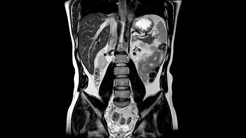
Test set: the reconstruction was tested on an independent set of images from several categories: a standard test brain image (taken from the ESPIRiT publically available demo code); magnitude abdomen MR images from the public domain (https://images.computerhistory.org/makesoftware/5.6_Abdominal-MRI.jpg); a natural magnitude image of a house; a multi-ellipse phantom image; and two complex-valued brain images acquired in our institution.

Additionally, MLN were compared to CascadeNet⁴⁷, based on single-channel Cartesian data, in order to match the provided implementation. 2 MLNs were tested, with training on HCP data, as described above, and on the knee data, as the one used by the CascadeNet. NRMSE values are reported.

Implementation

The networks were implemented in TensorFlow using a standard configuration (Adam optimizer with fixed learning rate (unless mentioned otherwise) of 0.002 and beta = 0.9, L₁ loss) on a desktop workstation with commercial GPU (NVIDIA GTX 1080 Ti with 11GB of memory). The networks were trained by applying the slice-specific B₀ field map and sensitivity maps.

Networks were implemented to perform complex-field operations. No activation layers were used. B₀ maps were calculated using the method of Cusack et al.⁴⁸. Coil sensitivity maps were calculated with BART’s ESPIRiT module⁴⁹ using default parameters, and software coil compression (SCC) of the experimental MRI data was done using SVD. For reference reconstruction, BART’s pics module³⁵ with manually optimized parameters was expanded with implementation accounting for B₀ correction with time-segmentation²⁸, using up to 15 time segments, equally spaced over the acquisition time. NUFT⁵⁰ was also calculated using gpuNUFFT⁵¹. The images were also reconstructed using either the sparseMRI package⁵, or L₁-CG-ESPIRiT with L₁-wavelet or split TV and L₁-wavelet regularization⁴⁹. Parameters were set manually to optimize image quality.

The ASL data was motion corrected using ANTs⁵² and brain extracted using FSL BET⁵³ following which perfusion tSNR maps were computed.

Memory and performance considerations

The memory requirements for training are linear with the size of the two tensors calculated (the k- and I- side tensors). In these experiments, we also loaded the database to the GPU memory for increased performance. For the real-data spiral trajectories, training was run for 2 hours per instance, which achieved convergence. Inference was done by directly applying the calculated kernels.

NUFFT for MRI under field inhomogeneities

For the sake of completeness, we briefly summarize the approach developed in^27,28,46,50 for MR image-to-signal transform under field inhomogeneities and its use for image reconstruction, which was used for reference reconstruction as detailed above and laid the basis for the suggested networks’ topologies.

Let I be an image, and F_u be the non-uniform Fourier transform according to the given trajectory, acquiring N data points in acquisition duration T. Set L to be a (small) number of “time-segments”, separated by duration $\Delta =T{/}L$. The local phase evolution due to the field inhomogeneity at time-segment l, i.e. after lΔ acquisition time units, is ${P}_{l}(r)={e}^{-i{B}_{0}(r)l\Delta }$, and the image affected by the phase evolution is ${D}_{l}=I\odot {P}_{l}$, where $\odot$ marks element-wise Hadamard multiplication. Let G be an Nx(L + 1) matrix containing interpolation coefficients for each (discrete) timepoint (e.g. linear of Hanning interpolation, or interpolation matrix optimized for the specific case, such as via the min-max approach²⁸. The signal at time t can be approximated by $\hat{s}=\mathop{\sum }\limits_{j=0}^{L}{F}_{u}\{I\odot {P}_{j}\}\odot {G}_{j}.$ A NUFFT operation can be effectively and accurately approximated by (sparse) matrix multiplication of the FFT of the image with a precalculated coefficients matrix C, which is non-zero for a row corresponding to spatial frequencies f_x,f_y only in a window around those frequencies⁵⁰.

Conversely, The input to the network is the data, put into the 4-dimensional tensor S, of the form, [kRO,kPE, Neighbor, Channel]. That is, at each kx,ky location, the data from the NNeighbors nearby (non-Cartesian) acquired points is put into the tensor S.

The system only trains two tensors, H of size [RO,PE,NNeighbors, Nch, NTS] and M of size [RO,PE,NTS].

The regridded “segments (?)” are ${K}_{i,j,t}={\sum }_{n,c}{S}_{i,j,n,c}{H}_{i,j,n,c,t}$, and the reconstructed image is ${\hat{I}}_{i,j}={\sum }_{t}{K}_{i,j,t}{M}_{i,j,t}$.

While the 2nd multiplication is done pixel-wise in image-space, H is a non-Cartesian GRAPPA-like operation, i.e. a localized regridding kernel.

The generalization to multi-channel data is trivial and was implemented in the suggested networks.

References

Mardani, M., Gong, E., Cheng, J. Y. & Vasanawala, S. Deep generative adversarial networks for compressed sensing automates MRI. IEEE Trans. Med. Imaging 38, 167–179 (2019).
Han, Y. & Ye, J. C. k-Space Deep Learning for Accelerated MRI. IEEE Trans. Med. Imaging Early access (2019).
Schlemper, J., Caballero, J., Hajnal, J. V., Price, A. N. & Rueckert, D. A deep cascade of convolutional neural networks for dynamic MR image reconstruction. IEEE Trans. Med. Imaging 37, 491–503 (2018).
Zhu, B., Liu, J. Z., Cauley, S. F., Rosen, B. R. & Rosen, M. S. Image reconstruction by domain-transform manifold learning. Nature 555, 487–492 (2018).
Lustig, M., Donoho, D. & Pauly, J. M. Sparse MRI: The application of compressed sensing for rapid MR imaging. Magn. Reson. Med. 58, 1182–1195 (2007).
Pruessmann, K. P., Weiger, M., Scheidegger, M. B. & Boesiger, P. SENSE: sensitivity encoding for fast MRI. Magn. Reson. Med. 42, 952–962 (1999).
Griswold, M. A. et al. Generalized autocalibrating partially parallel acquisitions (GRAPPA). Magn. Reson. Med. 47, 1202–1210 (2002).
Yang, Y., Sun, J., Li, H. & Xu, Z. ADMM-Net: A deep learning approach for compressive sensing MRI. Advances in Neural Information Processing Systems 29 10–18 (Curran Associates, Inc., 2014).
Hammernik, K. et al. Learning a variational network for reconstruction of accelerated MRI data. Magn. Reson. Med. 79, 3055–3071 (2018).
Baldi, P. F. & Hornik, K. Learning in linear neural networks: a survey. IEEE Trans. Neural Netw. 6, 837–858 (1995).
Saxe, A. M., McClelland, J. L. & Ganguli, S. Exact solutions to the nonlinear dynamics of learning in deep linear neural networks. Submitted to ICLR (2014).
Trabelsi, C. et al. Deep Complex Networks. International Conference on Learning Representations (2018).
Ma, D. et al. Magnetic resonance fingerprinting. Nature 495, 187–192 (2013).
Virtue, P., Yu, S. X. & Lustig, M. Better than real: Complex-valued neural nets for MRI fingerprinting. In 2017 IEEE International Conference on Image Processing (ICIP) 3953–3957 (IEEE, 2017), https://doi.org/10.1109/ICIP.2017.8297024.
Huang, F., Vijayakumar, S., Li, Y., Hertel, S. & Duensing, G. R. A software channel compression technique for faster reconstruction with many channels. Magn. Reson. Imaging 26, 133–141 (2008).
Howard, A. G., Zhu, M., Chen, B. & Kalenichenko, D. Mobilenets: Efficient convolutional neural networks for mobile vision applications. arXiv:1704.04861v1 [cs.CV] (2017).
Chollet, F. Xception: Deep Learning with Depthwise Separable Convolutions. in 2017 IEEE Conference on Computer Vision and Pattern Recognition (CVPR) 1800–1807 (IEEE, 2017). https://doi.org/10.1109/CVPR.2017.195.
Ivanov, D. et al. Comparison of 3T and 7T ASL techniques for concurrent functional perfusion and BOLD studies. Neuroimage 156, 363–376 (2017).
Ivanov, D., Poser, B. A., Huber, L., Pfeuffer, J. & Uludağ, K. Optimization of simultaneous multislice EPI for concurrent functional perfusion and BOLD signal measurements at 7T. Magn. Reson. Med. 78, 121–129 (2017).
Gregor, K. & LeCun, Y. Emergence of Complex-Like Cells in a Temporal Product Network with Local Receptive Fields. arXiv:1006.0448v1 [cs.NE] (2010).
Taigman, Y., Yang, M., Ranzato, M. & Wolf, L. DeepFace: Closing the Gap to Human-Level Performance in Face Verification. in 2014 IEEE Conference on Computer Vision and Pattern Recognition 1701–1708, https://doi.org/10.1109/CVPR.2014.220 (IEEE, 2014).
Sodickson, D. K. & Manning, W. J. Simultaneous acquisition of spatial harmonics (SMASH): fast imaging with radiofrequency coil arrays. Magn. Reson. Med. 38, 591–603 (1997).
Doneva, M. & Börnert, P. Automatic coil selection for channel reduction in SENSE-based parallel imaging. MAGMA 21, 187–196 (2008).
Buehrer, M., Pruessmann, K. P., Boesiger, P. & Kozerke, S. Array compression for MRI with large coil arrays. Magn. Reson. Med. 57, 1131–1139 (2007).
Zhang, T., Pauly, J. M., Vasanawala, S. S. & Lustig, M. Coil compression for accelerated imaging with Cartesian sampling. Magn. Reson. Med. 69, 571–582 (2013).
Seiberlich, N. et al. Non-Cartesian data reconstruction using GRAPPA operator gridding (GROG). Magn. Reson. Med. 58, 1257–1265 (2007).
Fessler et al. iterative image reconstruction for MRI with correction for magnetic field inhomogeneity. IEEE Trans. Signal Process. 53, 3393–3402 (2005).
Sutton, B. P., Noll, D. C. & Fessler, J. A. Fast, iterative image reconstruction for MRI in the presence of field inhomogeneities. IEEE transactions on medical imaging (2003).
Weller, D. S., Ramani, S. & Fessler, J. A. Augmented Lagrangian with variable splitting for faster non-Cartesian L1-SPIRiT MR image reconstruction. IEEE Trans. Med. Imaging 33, 351–361 (2014).
Cybenko, G. Approximation by superpositions of a sigmoidal function. Math. Control Signals Syst. 2, 303–314 (1989).
Hornik, K., Stinchcombe, M. & White, H. Multilayer feedforward networks are universal approximators. Neural Netw. 2, 359–366 (1989).
Montufar, G. F., Pascanu, R., Cho, K. & Bengio, Y. In Advances in Neural Information Processing Systems 27 (eds. Ghahramani, Z., Welling, M., Cortes, C., Lawrence, N. D. & Weinberger, K. Q.) 2924–2932 (Curran Associates, Inc., 2014).
Poole, B., Lahiri, S., Raghu, M., Sohl-Dickstein, J. & Ganguli, S. In Advances in Neural Information Processing Systems 29 (eds. Lee, D. D., Sugiyama, M., Luxburg, U. V., Guyon, I. & Garnett, R.) 3360–3368 (Curran Associates, Inc., 2016).
Schlemper, J. et al. dAUTOMAP: Decomposing AUTOMAP to Achieve Scalability and Enhance Performance. Proc. ISMRM (2019).
Uecker, M., et al Berkeley Advanced Reconstruction Toolbox. Proc. ISMRM (2015).
Alsop, D. C. et al. Recommended implementation of arterial spin-labeled perfusion MRI for clinical applications: A consensus of the ISMRM perfusion study group and the European consortium for ASL in dementia. Magn. Reson. Med. 73, 102–116 (2015).
Wang, Z., Bovik, A. C., Sheikh, H. R. & Simoncelli, E. P. Image Quality Assessment: From Error Visibility to Structural Similarity. IEEE Trans. on Image Process. 13, 600–612 (2004).
Van Essen, D. C. et al. The WU-Minn Human Connectome Project: an overview. Neuroimage 80, 62–79 (2013).
Kim, S. G. Quantification of relative cerebral blood flow change by flow-sensitive alternating inversion recovery (FAIR) technique: application to functional mapping. Magn. Reson. Med. 34, 293–301 (1995).
Wong, E. C., Buxton, R. B. & Frank, L. R. Quantitative imaging of perfusion using a single subtraction (QUIPSS and QUIPSS II). Magn. Reson. Med. 39, 702–708 (1998).
Hurley, A. C. et al. Tailored RF pulse for magnetization inversion at ultrahigh field. Magn. Reson. Med. 63, 51–58 (2010).
Williams, D. S., Detre, J. A., Leigh, J. S. & Koretsky, A. P. Magnetic resonance imaging of perfusion using spin inversion of arterial water. Proc Natl Acad Sci USA 89, 212–216 (1992).
Detre, J. A., Leigh, J. S., Williams, D. S. & Koretsky, A. P. Perfusion imaging. Magn. Reson. Med. 23, 37–45 (1992).
Teeuwisse, W. M., Brink, W. M. & Webb, A. G. Quantitative assessment of the effects of high-permittivity pads in 7 Tesla MRI of the brain. Magn. Reson. Med. 67, 1285–1293 (2012).
Kim, D., Adalsteinsson, E. & Spielman, D. M. Simple analytic variable density spiral design. Magn. Reson. Med. 50, 214–219 (2003).
Sutton, B. P., Noll, D. C. & Fessler, J. A. Fast, iterative, field-corrected image reconstruction for MRI. In Proceedings IEEE International Symposium on Biomedical Imaging 489–492, https://doi.org/10.1109/ISBI.2002.1029301 (IEEE, 2002).
Schlemper, J., Caballero, J., Hajnal, J. V., Price, A., & Rueckert, D. A Deep Cascade of Convolutional Neural Networks for MR Image Reconstruction. Information Processing in Medical Imaging (IPMI), (2017).
Cusack, R. & Papadakis, N. New robust 3-D phase unwrapping algorithms: application to magnetic field mapping and undistorting echoplanar images. Neuroimage 16, 754–764 (2002).
Uecker, M. et al. ESPIRiT–an eigenvalue approach to autocalibrating parallel MRI: where SENSE meets GRAPPA. Magn. Reson. Med. 71, 990–1001 (2014).
Fessler, J. A. On NUFFT-based gridding for non-Cartesian MRI. J. Magn. Reson. 188, 191–195 (2007).
Knoll, F., Schwarzl, A. & Diwoky, C. gpuNUFFT-an open source GPU library for 3D regridding with direct Matlab interface. Proc. ISMRM (2014).
Avants, B. B. et al. A reproducible evaluation of ANTs similarity metric performance in brain image registration. Neuroimage 54, 2033–2044 (2011).
Smith, S. M. Fast robust automated brain extraction. Hum. Brain Mapp. 17, 143–155 (2002).
Acknowledgements
This project was funded by NWO 016.VIDI 178.052 to B.A.P. Data was acquired at Scannexus BV, Maastricht, NL (www.scannexus.nl). The authors thankfully acknowledge the help of Dr. Dimo Ivanov with the ASL data acquisition and analysis, as well as Dr. Sriranga Kashyap for assistance with perfusion analysis and preparing the figures for this manuscript.
Author information
Authors and Affiliations
Contributions
G.L. conceived the D.L. approaches, implemented the M.R. sequences and reconstruction, acquired the data and wrote the paper. B.A.P. contributed to the M.R. sequences and writing of the paper.
Corresponding author
Ethics declarations
Competing interests
The authors declare no competing interests.
Additional information
Publisher’s note Springer Nature remains neutral with regard to jurisdictional claims in published maps and institutional affiliations.
Supplementary information
Rights and permissions
Open Access This article is licensed under a Creative Commons Attribution 4.0 International License, which permits use, sharing, adaptation, distribution and reproduction in any medium or format, as long as you give appropriate credit to the original author(s) and the source, provide a link to the Creative Commons license, and indicate if changes were made. The images or other third party material in this article are included in the article’s Creative Commons license, unless indicated otherwise in a credit line to the material. If material is not included in the article’s Creative Commons license and your intended use is not permitted by statutory regulation or exceeds the permitted use, you will need to obtain permission directly from the copyright holder. To view a copy of this license, visit http://creativecommons.org/licenses/by/4.0/.
About this article
Cite this article
Liberman, G., Poser, B.A. Minimal Linear Networks for Magnetic Resonance Image Reconstruction. Sci Rep 9, 19527 (2019). https://doi.org/10.1038/s41598-019-55763-x
Received:
Accepted:
Published:
Version of record:
DOI: https://doi.org/10.1038/s41598-019-55763-x