Abstract
This study introduces an innovative method for addressing the bearing fault detection problem in rotating machinery. The proposed approach integrates multi-feature extraction, advanced feature selection, and state-of-the-art classification techniques using convolutional neural network (CNN) models. Leveraging the comprehensive Fault Bearing Dataset from Case Western Reserve University (CWRU), continuous wavelet transforms (CWT) and CNNs are utilized for feature extraction. The methodology also incorporates machine learning model tuning through Tree-Structured Parzen Estimators (TPE) for optimal hyperparameter adjustment, ensuring high-performance classification. Experimental results, based on the ResNet-50-SVM hybrid model, showed the effectiveness of the proposed approach in achieving an impressive accuracy of 95.51%. This confirms that the proposed methodology represents a significant advancement in bearing fault detection, providing an effective solution for predictive and preventive maintenance in industrial applications.
Introduction
Motivation
Induction motors have long formed the core of industries in various fields because of their strong construction, high efficiency, and adaptability1,2. However, induction motors are not immune to a variety of faults that may cause severe operational interruptions and financial losses. For instance, approximately 10% of motor failures are caused by the rotor, while more than 40% are caused by bearings3,4. This creates a high demand for monitoring systems to detect early faults in order to reduce both losses in productivity as well as the costs of the repair and/or replacement of damaged equipment5. Conventional approaches applied for bearing fault detection, such as manual inspections, vibration analysis and statistical methods have been criticized for their limitations in terms of accuracy and adaptability to varying operating conditions6,7,8. Given these limitations, AI-driven techniques, particularly machine learning (ML) and deep learning (DL) methods, have been emerged as powerful alternatives for automated fault detection and diagnosis in rotating machinery8,9,10. However, these approaches necessitate precise tuning of the hyperparameters, particularly when the accuracy is a determining factor. Hence, the integration of efficient optimization techniques into machine learning models ensures that such a fault detection and diagnosis strategy is more accurate and adaptive to varying operating conditions. Within this context, this research presents an advanced ML framework for bearing fault diagnosis where various techniques are integrated to improve feature extraction and optimize hyperparameter tuning.
Literature review
Based on literature review, it is found that bearing fault detection methods can be categorized into four main groups11 which are (i) model-based, (ii) signal-based, (iii) data-driven, and (iv) hybrid techniques. Model-based strategies12,13 use mathematical models of the system to predict its behavior. Then, faults can be identified by comparing predicted outputs with actual system outputs. For instance, in12, bearing faults are modeled as time-varying rotor eccentricities, which result in distortions in the motor current. These distortions are analyzed to detect bearing faults. However, the applicability of such methods faces some difficulties when dealing with complex systems operating under variable conditions. Signal-based approaches are based on processing and interpretation of different signals, such as motor currents, vibration and acoustic signals to detect and analyze faults15. Generally, these approaches use techniques, like frequency analysis16, time-domain analysis17, and signal processing tools18 to detect and assess machine faults. In signal-based methods, signals are analyzed without requiring physical access to the internal components of the system. However, the performance of this kind of methods can be affected by varying operating conditions, such changes in the machine speed and load.
In contrast to the model-based and signal-based techniques, data-driven techniques utilize ML and AI algorithms to identify fault features and patterns19,20,21,22. These algorithms use large amount of historical and real-time data obtained through sophisticated data acquisition to detect faults with high accuracy. In various recent studies23,24,25, data-driven techniques were based on artificial neural networks (ANNs), since they are capable of learning complex data patterns. In these studies, it has been justified that ANNs can be used to diagnose various types of faults, including bearing and rotor faults, from the vibration and current signals. In other data-driven approaches, ML-based models including support vector machine (SVM)24, CNN26, deep transfer learning (DTL)27, and long short-term memory (LSTM)28 are widely used for fault diagnosis. Despite it was found that this group of techniques offers enhanced accuracy over the conventional approaches, each method has its own advantages and disadvantages, which must be carefully considered based on the specific application and operational requirements29. In recent years, various studies have focused on the development of hybrid techniques that combine multiple ML models approaches to achieve superior performance and accuracy of bearing fault detection models20,21,22. Table 1 presents some examples of various methods introduced in the literature review.
Study contributions
This research presents an efficient ML framework for bearing fault diagnosis integrating an improved feature extraction and classification strategy. The proposed framework enables early and accurate detection of bearing faults, reducing unexpected machinery failures and minimizing downtime in industrial applications. The main contributions of this study are summarized as follows:
-
In the proposed framework, an advanced hybrid strategy combining CNNs and CWTs functions is proposed as a deep feature extraction system instead of traditional methods that use single feature extraction and classification models. A TPE-based hyperparameter tuning mechanism is employed to simultaneously optimize the parameters of CNN and ML models, ensuring optimal fault detection classification.
-
The suggested method improves classification robustness by using various classifiers (SVM, KNN, RF, and DT) and ResNet50 for deep feature extraction. With an accuracy of 95.51%, the combination of ResNet50 and SVM outperforms traditional CNN models based on CWT.
-
The proposed methodology investigates different bearing faults across various operational conditions, thereby improving both model flexibility and robustness in handling operational faults. By incorporating DL and ML classifiers, the developed framework offers superior reliability, making it more robust and capable of performing effectively across diverse industrial settings beyond CNN-based approaches.
Materials and methods
The approach suggested in this study involves three main steps: (i) raw vibration data acquisition, (ii) application of CWTs to convert the data into time–frequency, and (iii) classification of the input data set as either healthy or faulty using CNN models and other ML algorithms. The entire proposed fault diagnosis system is depicted in Fig. 1. As shown in this figure, the system starts with the analysis of the raw vibration signals using CWT in order to produce the time–frequency images necessary for accurate fault identification. These images are then passed through a number of CNN models, including DenseNet201, Vgg19, and ResNet50 to draw out improved features that describe the state of the machinery. Another layer of features is then extracted and analyzed to differentiate between healthy and faulty states. The extracted features are analyzed using classifiers, including SVM, KNN, Random Forest (RF), and Decision Tree (DT). Examples of fault conditions adopted for the fault diagnosis are associated with the inner race (IR), outer race (OR) and ball faults in a bearing with 0.007-inch, 0.014-inch and 0.021-inch defects. These fault conditions are symbolized in Fig. 1 by IR_007, IR_014, IR_021, OR_007, OR_014, OR_021, BALL_007, BALL_014 and IR_021.
Data description
The need to improve the accuracy and reliability of bearing fault diagnosis has pushed researchers to look for new methods. In the current work, the complexities of fault recognition is addressed by using the Seeded Fault Bearing Dataset from CWRU bearing data center which is a widely recognized benchmark in bearing fault diagnosis datasets. The selection of the CWRU dataset is attributed to its high-quality data and unmistakable fault characteristics30. Indeed, the approach presented in30 takes place with reference to the three carefully developed unbalanced datasets that are subjected to diverse loads varying from 0 to 3 Hp. The essence of our experimentation lies in the mutual relationship between a 2-Hp reliance electric motor, a torque transducer, and a dynamometer, operating across a range of loads and motor speeds varying from 1730 to 1797 revolutions per minute (rpm). Taking advantage of the high accuracy of electro-discharge machining (EDM) technology, the proposed method incorporates single-point defects of various depths on the inner race, outer race, and rolling element of the experimental bearing. The fault diameters of 7 mils, 14 mils, and 21 mils define a range of fault conditions that push our method to distinguish the fine details of bearing health. Table 2 describes the characteristics of bearings for both healthy and faulty conditions.
The resulting compilation is an extensive dataset encompassing the characteristics of signals corresponding to healthy condition (HC), IRF, BF, and ORF. Notably, the ORF classification unfolds in three unique forms: ORF at the center, ORF at the orthogonal position, and ORF at the opposite position. Each variation introduces an additional level of intricacy to our diagnostic ensemble. Our investigation focuses on variable-length vibration acceleration signals, meticulously recorded at an impressive 48,000 samples per second (Hz) for drive-end bearings operating at 2 Hp and 1750 rpm. A specific spotlight shines on the ORF at the center variant unraveling the intricacies of fault recognition in this particular configuration. The fundamental arrangement of the experimental setup is depicted in Fig. 2.
Computational Cost Consideration and Key Fault Conditions Focus: Due to computational cost considerations, the analysis was limited to four key fault conditions with fault diameters of 0.007 inches. Even so, the results indicate strong classification accuracy and validate the proposed method.
Data processing in vibration signal analysis
When loading the vibration data for analyzing the signals corresponding to different bearing conditions, a significant step is triggered as shown in Fig. 3. This step involves segmentation, where the whole vibration signal is divided into smaller parts; in this case, the segments are of 1000 samples. The primary goal of segmentation is to find and define certain types of faults in the signal and to reduce the amount of computations for further analysis. One of the crucial elements of the procedure described in this paper is the use of the CWT for each segmented signal. After the CWT application, the outcomes are a matrix, which is then resized into a particular shape. This reshaped matrix is used to represent the time–frequency content of the signal and is then saved as an image. In vibration signal analysis, segmentation divides the continuous vibration signal into frames where faults can be detected locally. Let the original vibration signal be designated as x (t), and ‘t’ refers to time. The segmentation can be mathematically expressed as:
where \({x}_{i}\left(t\right)\) is the segmented signal. T is the segment length (e.g., 1000 samples). N is the total number of segments.
This step allows for time-localization of faults, optimizing computational load.
The CWT is able to convert the segmented vibration signal from time-domain to time–frequency domain thus provides information on both time and frequency. The CWT of a signal \(x(t)\) is defined as follows.
where \(a\) is the scale parameter (inversely related to frequency). \(b\) is the time-shift parameter. \({\psi }^{*}\) is the complex conjugate of the mother wavelet function ψ.
In this application, the CWT is utilized to capture localized time–frequency features of the vibration signal.
CNN model and tree-structured Parzen estimator for feature extraction
Tree-structured Parzen estimator for hyperparameter
The tree-structured Parzen estimator is a Bayesian optimization algorithm, sometimes called sequential model-based optimization. In the proposed methodology, a TPE is used to search the space of hyperparameters, including both the algorithmic and architectural ones. Algorithmic hyperparameters are learning rate and data normalization, while architectural hyperparameters include kernel size, stride, network operators, and other related settings, which will be described in detail later31.
The feature layer is used for classification and is presented as input for machine learning algorithms. This is because maximum accuracy can only be obtained if the parameters that are very essential for determining the classification accuracy have been identified. In our application, a TPE is used in the training phase to identify the proper hyperparameters for each ML algorithm. Different algorithms require specific hyperparameter tuning to optimize performance. For instance, for KNN, hyperparameters include the distance metric and the number of neighbors, while for SVM, they include box constraints (C), the coding method, and the kernel type. DT depends on minimum leaf size, kernel width, and distribution type, while RF has its own hyperparameters.
The values of these hyperparameters, selected through TPE, are given in Table 3. After that the optimization of the parameter values is made and then the training and testing phase is also performed. The training phase of every ML algorithm used in the study adopts a stopping criterion based on the number of iterations allowed.
The use of this approach in concert with other advanced methods such as support vector machines and neural networks has been found to help facilitate the optimization of the model32. TPE uses two different probability distributions—one for favorable configuration and the other for the unfavorable one. Below is the simplified TPE formula.
Let’s denote the hyperparameters as \(x\), the objective function as \((x)\), and the hyperparameter space as \(X\). The goal is to find the optimal set of hyperparameters \({x}^{*}\) that maximizes or minimizes the objective function \(f\left(x\right)\) presented in Table 4.
CNN model and feature extraction
Numerous studies have explored the use of pre-trained CNN models to extract deep features for bearing fault diagnosis. In this study, after extracting deep features from CNN models, a feature selection mechanism is employed to ensure that only the most relevant features contribute to the classification process, thereby improving model accuracy and efficiency. In this study, TPE-based hyperparameter tuning is utilized not only for optimizing machine learning model parameters but also for selecting the most informative features. Indeed, this approach optimizes the ML model parameters while simultaneously influencing feature selection by fine-tuning the model to emphasize the most discriminative features for fault classification.
Researchers have also investigated transfer learning techniques and multiscale CNN architectures to enhance fault diagnosis in rotating machinery under varying conditions32. Moreover, the use of pre-trained CNN models in fault detection has gained traction, offering improved performance in identifying mechanical failures33. Additionally, converting vibration signals into RGB images and applying multichannel multiscale CNNs have shown promising results in detecting bearing faults more effectively34.
Furthermore, the dynamics modeling of bearings with defects and the direct transfer learning from simulation to test bench for bearing fault diagnosis have been performed, proving the CNN’s ability to extract deep features for fault diagnosis35. Also, based on 1-D adder neural networks and bidirectional LSTM (BLSTM) models in intelligent fault diagnosis of bearings, the potential of CNNs in deep feature extraction for fault diagnosis has been shown in36,37. In addition, the non-local 1D-CNNs are employed, and the collaboration of CNN and GAN for bearing fault diagnosis has also exhibited the ability to capture long range dependencies and address the problem of small sample size in fault diagnosis38,39. Moreover, the selection of dual attention dense convolutional networks and short-time Fourier transform in combination with CNN for intelligent fault diagnosis and remained useful life prediction of rolling bearings again highlights the feature extraction ability of CNNs for bearing fault diagnosis41,41.
In the following several works, the extensive utilization and successful application of pre-trained CNN models for deep feature extraction in bearing fault diagnosis are illustrated, which could be used for capturing the extensive and complex fault features as well as facilitating fault identification. In this study, we have used the following approach: we are using deep features derived from a standard CNN as input to multiple machine learning techniques. The chosen algorithms are KNN, DT (DT), RF, and SVM. The initial step involves adopting an existing pre-trained feature extractor CNN framework that has had prior performance in learning hierarchical and abstract features from heterogeneous datasets (VGG16, ResNet50, or Inception). After the feature extraction process, many necessary steps are performed on the dataset. The data set is then split into variable train and test sets to ensure valid model testing is done. After that, various other machine learning models are employed with the deep features extracted from the images.
Table 5 provides a concise overview of different CNN models used for deep feature extraction, including their input sizes, feature layers, and the number of features extracted.
Results and discussion
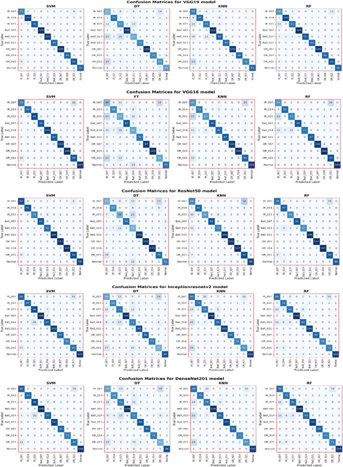
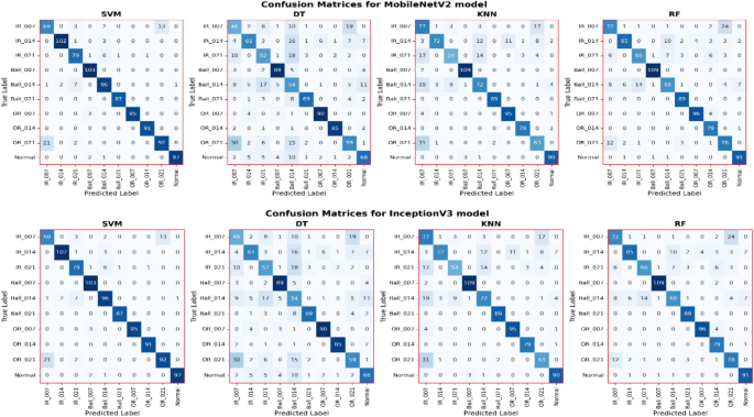
Time–frequency image representations are then classified using features acquired from seven different famous convolutional neural network models. Initial attempts to implement the DL algorithms are performed on a laptop with 16 GB of RAM and an Intel Core i5 CPU. In the training phase, the parameters affecting the accuracy of the various machine learning techniques are determined using the TPE method. These hyperparameters do not change during training as well as testing of the model on the test data set. The features extracted from each model are classified using four different ML techniques, including support vector machines, decision trees, k-nearest neighbors, and random forests. The confusion matrices for the given classification results are shown in Fig. 4 below. Apart from the confusion matrices, other measures that are derived from these matrices are computed and shown for the assessment of performance. These metrics served as numerical evaluations of the classification performance of the applied machine learning method.
The confusion matrices in Fig. 4 for the various models (VGG16, MobileNetV2, Inception V3, and DenseNet201) show distinct patterns of performance. The SVM model shows very good performance in most classes, especially in Ball_007, Ball_021, and Normal, where it only misclassifies a few instances of IR_007. The DT (Decision Tree) model performs well in classes like Ball_007 and Ball_021 but is poor in both Ball_014 and Normal. The KNN model performs quite well although it misclassifies IR_007 and Normal, while making a few mistakes in Ball_007 and Ball_021. Random Forest (RF) performs very well in all categories, but Ball_007 and Normal had the best results, while IR_007 and IR_021 had some errors. Most importantly, in the majority of the cases, SVM and KNN proved to be more effective than DT and RF on the other side, RF is stronger in stability and gives higher generalization as it has fewer errors of IR_007 and Ball_021. In general, these results reveal the dichotomy of accuracy and generalization, with SVM and KNN making fewer mistakes within certain categories, whilst RF exhibits greater resilience across all fault types and balance performance.
Table 6 demonstrates the effectiveness of machine learning methods, employing hyperparameters determined by the TPE for features produced from each CNN model. Comparative analysis shows that ResNet50 is the most accurate model, while SVM is identified as the most stable classification model. In particular, the structure of Res-Net50 with SVM allows achieving a high classification accuracy of 95.51%. This result is achieved through feature extraction from images using ResNet50 and using SVM for classification. The accuracy, sensitivity, and specificity for the Res-Net50-SVM structure are 0.9554, 0.9537, and 0.9542, respectively, while the MAE, RMSE, and R2 values are 0.21384, 1.1629, and 0.8374, respectively.
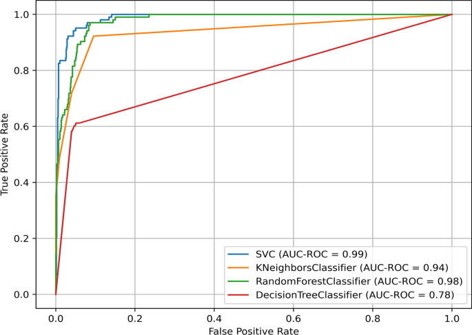
Figure 5 shows the ROC curve of Resnet50 for four different machine learning classifiers: SVM, KNN, RF, and DT. The AUC-ROC values of every classifier are also provided below. The ROC curve shows how well a classifier is performing, and the area under the ROC curve is a performance measure. The value of AUC-ROC also signifies a better classifier, and a higher value of it is preferred. In this figure, it can be seen that the AUC-ROC of the SVM model is 0.99, meaning the model is exceptionally accurate in predicting the outcome of a patient; the RF model has 0.98; the KNN has 0.94; and DT has 0.78, representing the accuracy of the model in predicting the outcome of a patient.
Figure 5 is the ROC curve of four classifiers, including SVC, KNeighborsClassifier, RandomForestClassifier, and DecisionTreeClassifier, which maps the TPR against the FPR. The AUC pairs these rates at different classification levels, illustrating the trade-off between them. The ideal curve for a good classifier will lie as near as possible to the top-left corner of the plot—a high TPR with a low FPR. In this figure, it can be seen that the SVM classifier has the highest value of AUC-ROC, with its curve closely located to the upper left corner of the graph. Other classifiers, such as RandomForestClassifier, yield an AUC-ROC of 0.98, and KNeighborsClassifier has a 0.94 AUC-ROC, while DecisionTreeClassifier has an AUC-ROC score of 0.78. Based on the results of this experiment, SVM is shown to be the best classifier among the three. The ROC curves for both the Random Forest (RF) and K-Nearest Neighbors (KNN) classifiers show good performance, which is evident from the curves being very close to the upper left-hand corner of the plot. Nonetheless, the ROC curve of the Decision Tree (DT) classifier is less effective and has a lower value of AUC-ROC. In general, it is evident from Fig. 5 above that the Support Vector Machine (SVM) has the highest AUC-ROC score, meaning that it is the best classifier for this task and is followed by the RF and KNN classifiers. However, the DT classifier is relatively poor when compared with the other models of classification.
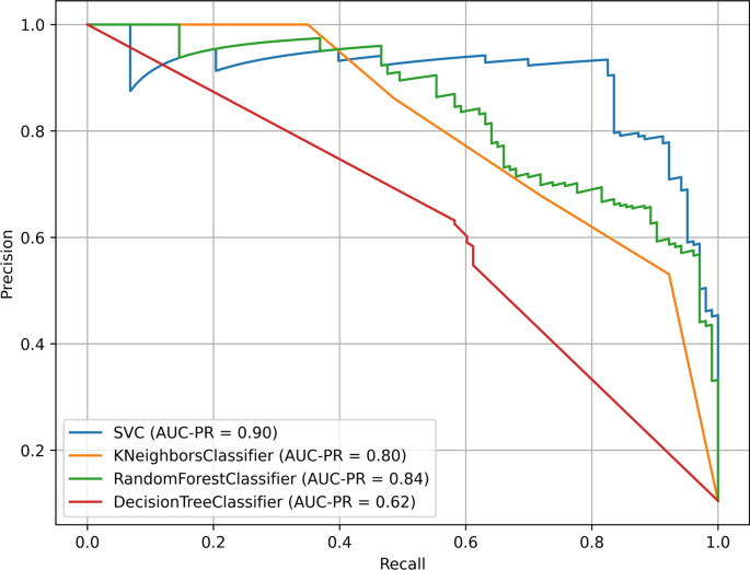
Figure 6 presents the precision-recall curve of Resnet50 for four classifiers: SVM, KNN, RF, and DT. The classification performance of each model is presented using the AUC-PR, the area under the curve of precision-recall. The AUC-PR value is higher if the model has better classification ability; the SVM model is 0.90, Random Forest 0.84, KNN 0.80, and Decision Tree 0.62.
The aperture is an approach that is used to represent the trade-off between precision and recall, where we have the precision-recall (PR) curve. Precision denotes the ratio of the true positive predictions to the total number of positive predictions made, while recall shows the number of actual positive cases correctly categorized amidst all the positive predictions made. From the PR curve in Fig. 6, the classifier with the highest precision and recall is the SVM classifier and is followed by the Random Forest and KNN, with the Decision Tree performing poorly on this classification task.
As it can be seen in Fig. 6, the precision-recall curve of the SVM classifier shows the highest precision for most of the recall values, indicating that the classifier performs the best for this task. The precision-recall curves for the RF and KNN are also good, but the precision-recall curve for the DT is slightly lower since DT has low precision for most recall values. From Fig. 5, it is clear that the SVM classifier is the most accurate classifier for this task, followed by the RF and KNN. The DT is not as good as the other classifiers. In summary, both Figs. 5 and 6 continually point out SVM as the best classifier for the given task, and it performs better in both ROC and precision-recall analyses. As for the rest of the algorithms, RF and KNN show much higher results than DT. These findings are useful in identifying the relative strengths of classifiers and, hence, in choosing the most appropriate model for a given classification task.
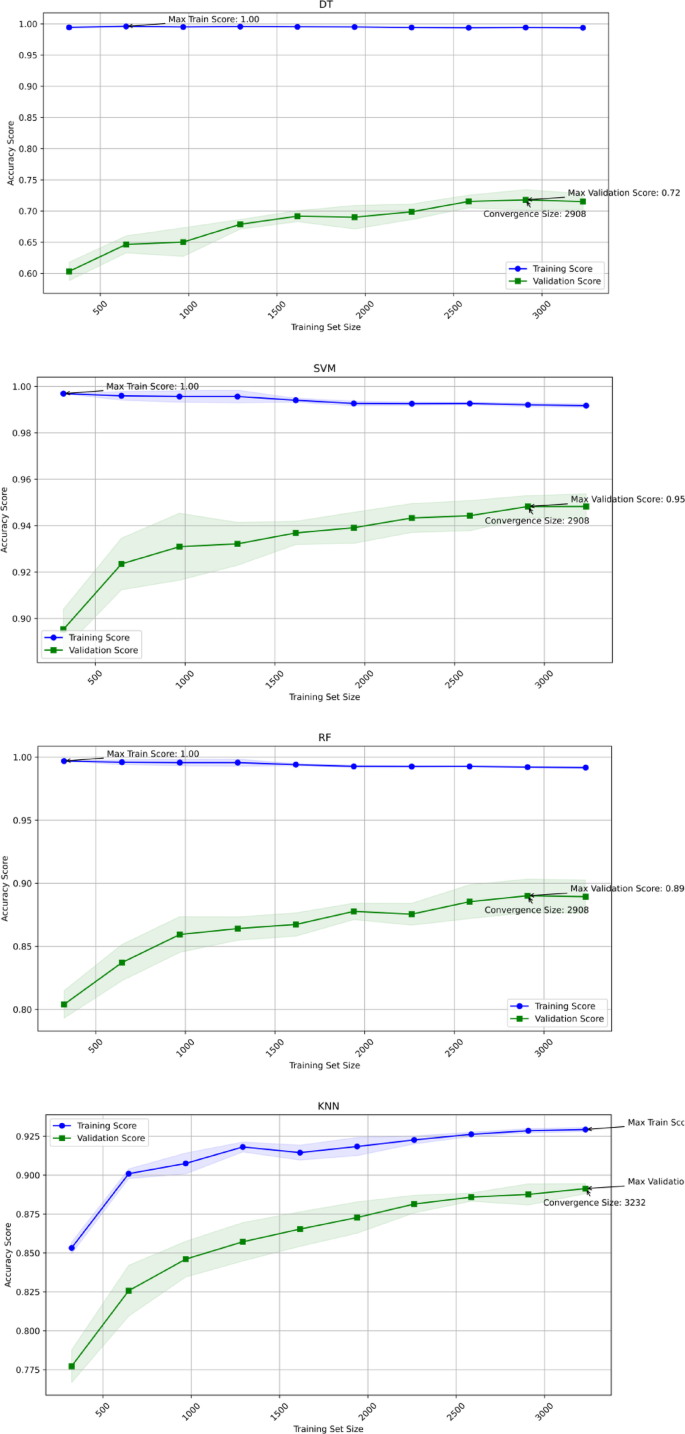
As shown in Fig. 7, the average accuracy scores of different machine learning classes, including Random Forest (RF), Support Vector Machine (SVM), K-Nearest Neighbors (KNN), and Decision Tree (DT), trained by a dataset using the ResNet50 structure are presented. The plots illustrate how training and validation accuracy evolve as the training set size increases, with accuracy values ranging from 0 to 1, where 1 represents perfect classification.
As we can see from this figure, the RF model can reach a maximum training accuracy of 0.99 when the training size is 3142, and the validation score oscillates around 0.92. The SVM classifier also achieves a good training accuracy of 0.99 and a validation score of 0.95 when the training set of 2195 is used, which shows better generalization. The KNN model has the maximum training accuracy of 0.94, but the validation accuracy converges to 0.84, meaning that the model is still good. Nevertheless, the DT model, which has received a nearly perfect training accuracy of 0.99, has many problems with overfitting. It is to be noted that the validation accuracy of the model begins at approximately 0.6 and increases to only 0.81. The difference between training and validating accuracy shows that, although the DT model achieves high accuracy on the training set, its performance is significantly lower on new data. However, the SVM and RF models are much better balanced between training and validation performance, with small differences between the scores obtained, which means better generalization. However, the KNN algorithm is only average, with training and validation scores climbing as the dataset size increases with the final validation accuracy of 0.91 at convergence. In general, the results indicate that all the models yield good training accuracy, but the SVM and RF classifiers are the most generalized, followed by KNN, while DT may have a little problem with overfitting.
The method was tested on a more complex dataset containing different operating conditions like loads and motor speeds (1797, 1772, 1750, and 1730 rpm) where torque values changed from 0 to 3 HP. There were 4 primary defects along with their respective fault diameters (inner race, outer race, and ball defects) of 0.007 inches. Although there were some limitations due to computation expense, the results showed very powerful multi-model classification. In particular, SVM yielded 100 percent accuracy, while KNN and RF models each reached 99% accuracy. DT showed a 92% accuracy which indicates the ability of the method to classify fault conditions. It can be concluded that the proposed methods work for various fault types and operating conditions and can therefore guarantee dependable diagnosis of faults.
The primary computational complexity arises during the search and selection phase, where the optimal CNN architecture and hyperparameters are determined using TPE. This phase involves computational overhead due to extensive model evaluations and optimizations. However, once the optimal configuration is identified, the final deployed model-ResNet-50 combined with SVM operates with significantly reduced complexity. ResNet-50, a pre-trained deep learning model, efficiently extracts features, while SVM ensures robust classification with lower computational cost compared to fully end-to-end deep learning models. This trade-off allows the proposed approach to maintain high detection accuracy while remaining computationally efficient for practical applications.
Comparison with some previous studies
Table 7 presents a comparison between the actual study and some previous works. In contrast to prior studies that have achieved higher rates, this method brings a new approach by combining CWT with feature extraction and hyperparameter tuning using TPE. This hybrid method not only increases classification performance but also improves generalization across multiple classes. Based on the model results, it is rated to be very robust because it achieves a classification accuracy of 95.51%. Because of this, the proposed framework can be considered more useful and dependable than models that focus on achieving the highest accuracy, thus making the methodology more applicable to real-world problems. In fact, accuracy alone does not fully determine the superiority of a method.
Study outcomes and limitations
The results of the proposed approach show that the accuracy rate is 95.51% when the multimodal feature extraction techniques are used in DL models like ResNet50-SVM. To validate its generalizability for different operating conditions, the proposed approach is tested on datasets covering different types of fault conditions including, inner race, outer race, and ball faults. A combination of different operational conditions including motor speeds 1797, 1772, 1750 and 1730 rpm, and torque levels ranging from 0 to 3 HP are employed to validate the robustness of the models. Despite its high accuracy, the real-time applicability of the approach remains untested, which may present challenges in practical deployment. Additionally, while the model demonstrates strong performance within the experimental dataset, variations among different rotating machines could affect its applicability, leading to inconsistent success rates across industrial environments.
According the obtained results and study limitations, future works will focus on evaluating the computational burden of the ResNet50-SVM hybrid model and comparing its performance with lightweight alternatives such as MobileNetV2. Additionally, efforts will be made to estimate the processing time required for data analysis to determine the feasibility of the proposed method for real-time applications. Further research will also involve applying these models to more complex datasets that encompass a wider range of operational parameters, including varying motor speeds and loads.
Conclusions
This paper presents an ML-based approach for bearing fault diagnosis, incorporating state-of-the-art feature extraction, hyperparameter tuning, and reliable classification. The approach integrates CWT with deep CNNs for feature extraction, providing a wide range of time–frequency features that enhance fault diagnosis accuracy. Furthermore, the hyperparameters of the classification models are optimized using TPE to ensure the best results. Time–frequency image representations of bearing signals were processed through various well-known deep learning models, including DenseNet201, Vgg19, and ResNet50. Features extracted from these models were analyzed and classified using different classifiers, such as SVM, KNN, RF, and DT. Experimental results indicated that ResNet50, combined with SVM, achieves the highest classification accuracy of 95.51%, outperforming other CNN-based feature extractors and classifiers. The proposed approach offers significant improvements over several methods presented in the literature by overcoming the limitations of controlled settings and single-feature classification models. Unlike traditional approaches, the proposed methodology enhances feature extraction techniques and improves model generalization and robustness. These advancements enable the model to more effectively handle the complex and dynamic fault patterns encountered in real-world applications which makes it more suitable for practical and industrial environments.
In future studies, it is planned to compare the proposed method with other types of signals, such as current signals and acoustic emission signals. Additionally, the effectiveness of this method will be evaluated in real-time fault diagnosis applications and its applicability will be explored for more diverse and complex machinery systems.
Data availability
The datasets used and analysed during the current study are available from the corresponding author on reasonable request.
References
Asad, B., Rassõlkin, A., Kallaste, A. & Belahcen, A. A survey of broken rotor bar fault diagnostic methods of induction motor. Electr. Control. Commun. Eng. 14(2), 117–124. https://doi.org/10.2478/ecce-2018-0014 (2018).
Ayhan, B., Trussell, H., Chow, M. & Song, M. On the use of a lower sampling rate for broken rotor bar detection with DTFT and AR-based spectrum methods. IEEE Trans. Ind. Electron. 55(3), 1421–1434. https://doi.org/10.1109/tie.2007.896522 (2008).
Al-Hashemi, S., Al-Dujaili, A. & Ajel, A. Speed control using an integral sliding mode controller for a three-phase induction motor. J. Tech. 3(3), 10–19. https://doi.org/10.51173/jt.v3i3.328 (2021).
Soother, D. & Daudpoto, J. A brief review of condition monitoring techniques for the induction motor. Trans. Can. Soc. Mech. Eng. 43(4), 499–508. https://doi.org/10.1139/tcsme-2018-0234 (2019).
Pu, S., Zheng, C., Vagapov, Y., Davydova, A. & Lupin, S. Broken bar fault diagnosis for induction machines under load variation condition using discrete wavelet transform. In Proceedings of IEEE East-West Design & Test Symposium (EWDTS 2014), Kiev, 1–4. https://doi.org/10.1109/EWDTS.2014.7027059 (2014).
Ayaz, E. A review study on mathematical methods for fault detection problems in induction motors. Balkan J. Electr. Comput. Eng. 2(3), 156–165. https://doi.org/10.17694/bajece.21387 (2014).
Burriel-Valencia, J., Puche-Panadero, R., Martínez-Román, J., Sapena-Bañó, Á. & Pineda-Sánchez, M. Fault diagnosis of induction machines in a transient regime using current sensors with an optimized slepian window. Sensors. 18(1), 146. https://doi.org/10.3390/s18010146 (2018).
Singh, E. Evaluation of bearing fault detection on different _k-folds using deep learning ensemble models. Int. J. Recent Innov. Trends Comput. Commun. 11(9), 1395–1401. https://doi.org/10.17762/ijritcc.v11i9.9104 (2023).
Drakaki, M., Karnavas, Y., Karlis, A., Chasiotis, I. & Tzionas, P. Study on fault diagnosis of broken rotor bars in squirrel cage induction motors: a multi-agent system approach using intelligent classifiers. IET Electr. Power Appl. 14(2), 245–255. https://doi.org/10.1049/iet-epa.2019.0619 (2020).
Toma, R., Prosvirin, A. & Kim, J. Bearing fault diagnosis of induction motors using a genetic algorithm and machine learning classifiers. Sensors. 20(7), 1884. https://doi.org/10.3390/s20071884 (2020).
Kiakojouri, A., Lu, Z., Mirring, P., Powrie, H. & Wang, L. A generalised intelligent bearing fault diagnosis model based on a two-stage approach. Machines. 12, 77. https://doi.org/10.3390/machines12010077 (2024).
Wang, C., Wang, M., Yang, B. & Song, K. A model-based method for bearing fault detection using motor current. J. Phys. Conf. Ser. 1650, 032130. https://doi.org/10.1088/1742-6596/1650/3/032130 (2020).
Zhang, S. et al. Model-based analysis and quantification of bearing faults in induction machines. IEEE Trans. Ind. Appl. 56(3), 2158–2170. https://doi.org/10.1109/TIA.2020.2979383 (2020).
Maliuk, A. S., Prosvirin, A. E., Ahmad, Z., Kim, C. H. & Kim, J. M. Novel bearing fault diagnosis using gaussian mixture model-based fault band selection. Sensors. 21, 6579. https://doi.org/10.3390/s21196579 (2021).
Kilickaya, S. & Eren, L. Bearing fault detection in adjustable speed drives via self-organized operational neural networks. Electr. Eng. https://doi.org/10.1007/s00202-024-02764-3 (2024).
Cheng, Y., Zou, D., Zhang, W. & Wang, Z. A hybrid time-frequency analysis method for railway rolling-element bearing fault diagnosis. J. Sens. 2019, 8498496. https://doi.org/10.1155/2019/8498496 (2019).
Zhang, C. et al. Time-domain sparsity-based bearing fault diagnosis methods using pulse signal-to-noise ratio. IEEE Trans. Instrum. Meas. 73, 3516804. https://doi.org/10.1109/TIM.2024.3375978 (2024).
Sun, S., Zhang, S. & Wang, W. A new monitoring technology for bearing fault detection in high-speed trains. Sensors. 23, 6392. https://doi.org/10.3390/s23146392 (2023).
Iunusova, E. et al. Early fault diagnosis in rolling element bearings: comparative analysis of a knowledge-based and a data-driven approach. J. Intell. Manuf. 35, 2327–2347. https://doi.org/10.1007/s10845-023-02151-y (2024).
Umar, M., Siddique, M. F., Ullah, N. & Kim, J.-M. Milling machine fault diagnosis using acoustic emission and hybrid deep learning with feature optimization. Appl. Sci. 14, 10404. https://doi.org/10.3390/app142210404 (2024).
He, Y., Fang, H., Luo, J., Pang, P. & Yin, Q. A hybrid method for fault diagnosis of rolling bearings. Meas. Sci. Technol. 35(12), 125012. https://doi.org/10.1088/1361-6501/ad774d (2024).
Huang, Y. et al. A hybrid deep learning network for diagnosing multipoint faults in rolling bearings under variable operating conditions. J. Mech. Sci. Technol. 38, 5989–6003. https://doi.org/10.1007/s12206-024-1018-8 (2024).
Kim, M., Lee, J., Wang, D. & Lee, I. Induction motor fault diagnosis using support vector machine, neural networks, and boosting methods. Sensors. 23(5), 2585. https://doi.org/10.3390/s23052585 (2023).
Kumar, R. & Anand, R. S. Bearing fault diagnosis using multiple feature selection algorithms with SVM. Prog. Artif. Intell. 13, 119–133. https://doi.org/10.1007/s13748-024-00324-1 (2024).
Purwahyudi, B. Recurrent neural network (RNN) based bearing fault classification of induction motor employed in home water pump system. Indones. J. Electr. Eng. Comput. Sci. 3(1), 405–412. https://doi.org/10.54732/jeecs.v3i1.148 (2018).
Abdelmaksoud, M., Torki, M., El-Habrouk, M. & Elgeneidy, M. Convolutional-neural-network-based multi-signals fault diagnosis of induction motor using single and multi-hannels datasets. Alex. Eng. J. 73, 231–248. https://doi.org/10.1016/j.aej.2023.04.053 (2023).
Kumar, P., Kumar, P., Hati, A. & Kim, H. Deep transfer learning framework for bearing fault detection in motors. Mathematics. 10(24), 4683. https://doi.org/10.3390/math10244683 (2022).
Wang, Q., Sun, Z., Zhu, Y., Li, D. & Ma, Y. A fault diagnosis method based on an improved diffusion model under limited sample conditions. PLoS ONE 19(9), e0309714. https://doi.org/10.1371/journal.pone.0309714 (2024).
Soomro, A. A. et al. Insights into modern machine learning approaches for bearing fault classification: A systematic literature review. Results Eng. 23, 102700. https://doi.org/10.1016/j.rineng.2024.102700 (2024).
Chen, Z., Gryllias, K. & Li, W. Intelligent fault diagnosis for rotary machinery using transferable convolutional neural network. IEEE Trans. Ind. Inform. 16(1), 339–349. https://doi.org/10.1109/tii.2019.2917233 (2020).
Xu, M., Gao, J., Zhang, Z. & Wang, H. Bearing-fault diagnosis with signal-to-rgb image mapping and multichannel multiscale convolutional neural network. Entropy 24(11), 1569. https://doi.org/10.3390/e24111569 (2022).
Tang, J. et al. Bearings intelligent fault diagnosis by 1-D adder neural networks. J. Dyn. Monit. Diagn. 1(3), 160–168. https://doi.org/10.37965/jdmd.2022.30 (2022).
You, D. et al. Intelligent fault diagnosis of bearing based on convolutional neural network and bidirectional long short-term memory. Shock Vib. 2021, 7346352. https://doi.org/10.1155/2021/7346352 (2021).
Wang, H., Liu, Z. & Ai, T. Long-range dependencies learning based on non-local 1d-convolutional neural network for rolling bearing fault diagnosis. J. Dyn. Monit. Diagn. 1(3), 148–159. https://doi.org/10.37965/jdmd.2022.53 (2022).
Ruan, D., Song, X., Gühmann, C. & Yan, J. Collaborative optimization of CNN and GAN for bearing fault diagnosis under unbalanced datasets. Lubricants. 9(10), 105. https://doi.org/10.3390/lubricants9100105 (2021).
Su, J. et al. Dual attention dense convolutional network for intelligent fault diagnosis of spindle-rolling bearings. J. Vib. Control. 27(21–22), 2403–2419. https://doi.org/10.1177/1077546320961918 (2020).
Zhou, S., Xiao, M., Bartoš, P., Filip, M. & Geng, G. Remaining useful life prediction and fault diagnosis of rolling bearings based on short-time fourier transform and convolutional neural network. Shock Vib. 2020, 8857307. https://doi.org/10.1155/2020/8857307 (2020).
Wen, L., Li, X. & Gao, L. A transfer convolutional neural network for fault diagnosis based on ResNet-50. Neural Comput. Appl. 32(10), 6111–6124. https://doi.org/10.1007/s00521-019-04097-w (2019).
Hou, L., Jiang, R., Tan, Y. & Zhang, J. Input feature mappings-based deep residual networks for fault diagnosis of rolling element bearing with complicated dataset. IEEE Access. 8, 180967–180976. https://doi.org/10.1109/access.2020.3028465 (2020).
Wu, Q., Zhu, Z., Tang, J. & Xia, Y. Fault diagnosis of printing press bearing based on deformable convolution residual neural network. Netw. Heterog. Media. 18(2), 622–646. https://doi.org/10.3934/nhm.2023027 (2023).
Ullah, Z., Lodhi, B. A. & Hur, J. Detection and identification of demagnetization and bearing faults in PMSM using transfer learning-based VGG. Energies 13(15), 3834. https://doi.org/10.3390/en13153834 (2020).
Li, Y., Tang, B., Jiang, X. & Yi, Y. Bearing fault feature extraction method based on GA-VMD and center frequency. Math. Probl. Eng. 2022, 2058258. https://doi.org/10.1155/2022/2058258 (2022).
Chen, Y. et al. ACDIN: Bridging the gap between artificial and real bearing damages for bearing fault diagnosis. Neurocomputing 294, 61–71. https://doi.org/10.1016/j.neucom.2018.03.014 (2018).
Yang, X. et al. A hybrid deep-learning model for fault diagnosis of rolling bearings. Measurement 169, 108502. https://doi.org/10.1016/j.measurement.2020.108502 (2021).
Funding
This research has been funded by the Deanship of the Scientific Research of the University of Ha’il, Saudi Arabia (project: RG-24 158).
Author information
Authors and Affiliations
Contributions
Conceptualization, K.A., M.B.B, M.N., I.M. and T.G.; methodology, K.A., A.K., B.M.A. and A.A.; software, M.B.B., I.M., A.A. and A.A.; validation, A.K and B.M.A.; formal analysis, T.G and A.A.; investigation, T.G. and A.A.; writing—original draft preparation, K.A., M.B.B., M.N., A.K., I.M., T.G., B.M.A., A.A. and A.A.; supervision, A.K.; project administration, T.G.; funding acquisition, T.G. All authors reviewed the manuscript.
Corresponding author
Ethics declarations
Competing interests
The authors declare no competing interests.
Additional information
Publisher’s note
Springer Nature remains neutral with regard to jurisdictional claims in published maps and institutional affiliations.
Rights and permissions
Open Access This article is licensed under a Creative Commons Attribution-NonCommercial-NoDerivatives 4.0 International License, which permits any non-commercial use, sharing, distribution and reproduction in any medium or format, as long as you give appropriate credit to the original author(s) and the source, provide a link to the Creative Commons licence, and indicate if you modified the licensed material. You do not have permission under this licence to share adapted material derived from this article or parts of it. The images or other third party material in this article are included in the article’s Creative Commons licence, unless indicated otherwise in a credit line to the material. If material is not included in the article’s Creative Commons licence and your intended use is not permitted by statutory regulation or exceeds the permitted use, you will need to obtain permission directly from the copyright holder. To view a copy of this licence, visit http://creativecommons.org/licenses/by-nc-nd/4.0/.
About this article
Cite this article
Alqunun, K., Bechiri, M.B., Naoui, M. et al. An efficient bearing fault detection strategy based on a hybrid machine learning technique. Sci Rep 15, 18739 (2025). https://doi.org/10.1038/s41598-025-02439-4
Received:
Accepted:
Published:
Version of record:
DOI: https://doi.org/10.1038/s41598-025-02439-4

