Figure 1

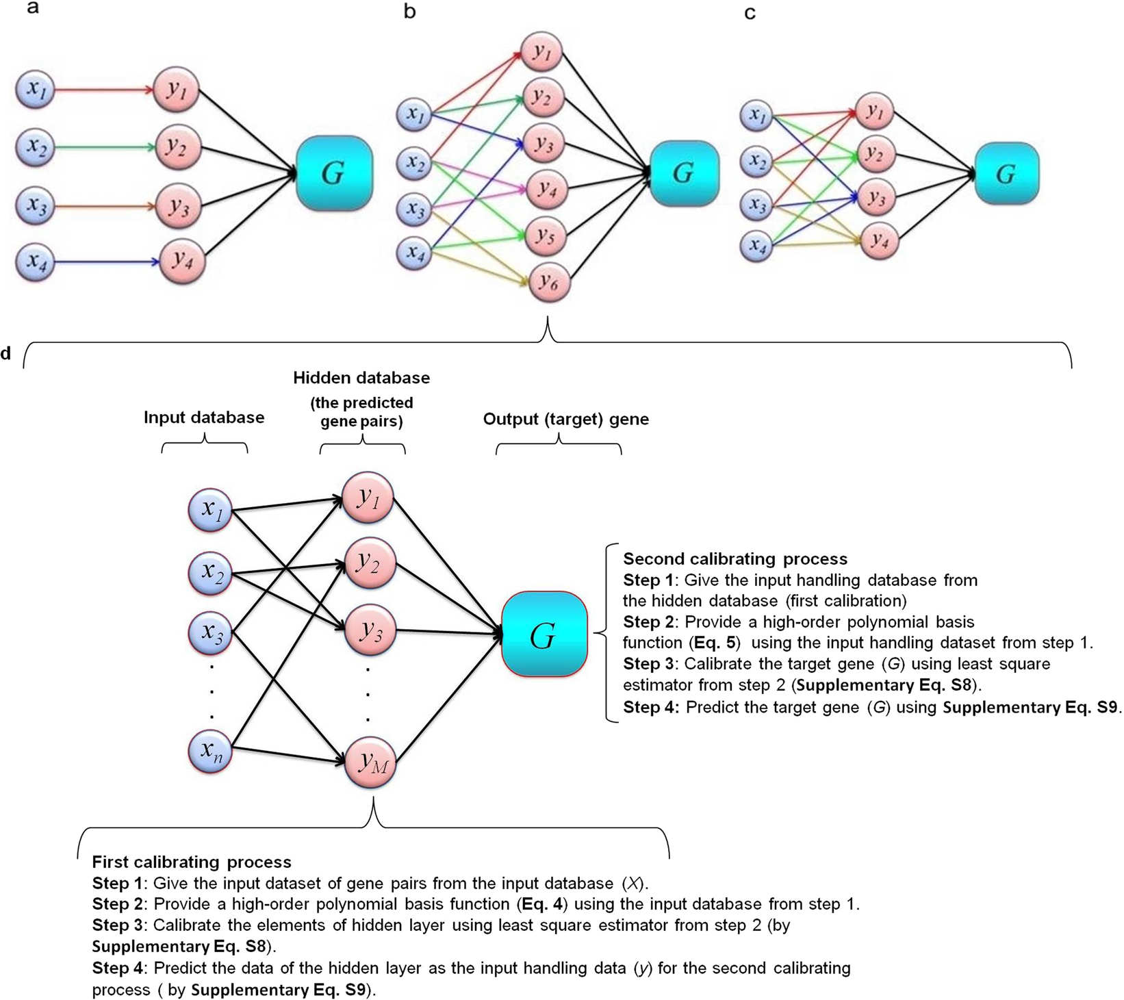
Schematic view of the different input gene sets for the hidden layer of MLRSM. (a) Scenario 1: the one-input dataset (x1) (for example, the gene expression data of TNFA) was used to calibrate the hidden predicted gene (y1). (b) Scenario 2: the two-input dataset (x1 and x2) (for example, the co-expression data of TNFA and IL1B) was used to calibrate the hidden predicted gene (y1). (c) Scenario 3: the three-input dataset (x1, x2, and x3) (for example, the gene expression data of TNFA, IL1B, and IL4) was applied for calibrating the elements of the hidden layer (y1). Then, y1 as a new input data was used for predicting the output/target gene (G) (for example, TLR4); and (d) this part provides a detail of the scenario 2. At the first calibration process, the hidden layer (y1 to ym) of the model was calibrated using the input genes (x1 to xn). Next, the output gene (G) was calibrated based on the calibrated dataset (the hidden layer) (y1 to ym). So, the second calibrating process was utilized to predict the output gene expression (G). Also, the data of the hidden layer of this model (gene pairs) was employed to construct Fig. 5a–e (the relationship between the co-expression of gene pairs and the output gene expression). The total elements in the hidden layer (M) were calculated based on the number of input genes (NS) and the total number of genes (n) as \(M=\frac{n!}{(n-NS)!NS!}\) where! is the factorial operator and NS ≤ n. So, the elements of the hidden layer were computed M = 4 for scenario 1 based on n = 4 and NS = 1 (i.e. \(M=\frac{n!}{(n-NS)!NS!}=\frac{4!}{(3)!\,1!}=4\)); M = 6 for scenario 2 based on n = 4; and NS = 2 and M = 4 for scenario 3 based on n = 4 and NS = 3.
