Noisy quantum trees: infinite protection without correction

Abstract

We study quantum networks with tree structures, in which information propagates from a root to leaves. At each node in the network, the received qubit unitarily interacts with fresh ancilla qubits, after which each qubit is sent through a noisy channel to a different node in the next level. Therefore, as the tree depth grows, there is a competition between the irreversible effect of noise and the protection against such noise achieved by the delocalization of information. In the classical setting, where each node simply copies the input bit into multiple output bits, this model has been studied as the broadcasting or reconstruction problem on trees, which has broad applications. In this work, we study the quantum version of this problem. We consider a Clifford encoder at each node that encodes the input qubit in a stabilizer code, along with a single qubit Pauli noise channel at each edge. Such noisy quantum trees describe a scenario in which one has access to a stream of fresh (low-entropy) ancilla qubits, but cannot perform error correction. Therefore, they provide a different perspective on quantum fault tolerance. Furthermore, they provide a useful model for describing the effect of noise within the encoders of concatenated codes. We prove that above certain noise thresholds, which depend on the properties of the code such as its distance, as well as the properties of the encoder, information decays exponentially with the depth of the tree. On the other hand, by studying certain efficient decoders, we prove that for codes with distance d ≥ 2 and for sufficiently small (but non-zero) noise, classical information and entanglement propagate over a noisy tree with infinite depth. Indeed, we find that this remains true even for binary trees with certain 2-qubit encoders at each node, which encodes the received qubit in the binary repetition code with distance d = 1.

Introduction

Overcoming noise and decoherence in quantum systems is the biggest challenge for quantum information technology. Understanding how these undesirable phenomena affect storage, communication and processing of quantum information is a problem with broad interest¹. Beyond these applications, understanding the competition between entanglement generation and noise in quantum circuits is a fundamental problem in many-body physics that has attracted significant attention in recent years^2,3,4,5.

Classically, the study of noisy circuits traces back to von Neumann when he proved the first threshold theorem for fault-tolerant computation using noisy elements⁶. In subsequent decades, Pippenger and others further developed this into a theory of noisy circuits^7,8,9,10. A particularly interesting and useful model for the propagation of classical information is broadcasting on noisy trees (see, e.g.,^11,12). A broad class of classical processes – both natural and artificial – can be modeled as such trees. Applications include broadcasting networks, reconstruction in genetics, and Ising models in statistical physics^11,12,13,14.

Here we consider a basic version of this problem: at a distinguished node, called the root of the tree, a bit of information is received and then it is sent to b other nodes in the next level. Then, each node in the next level sends the received bit to b other nodes in the next level, and so on. Now suppose each link between the nodes at two successive levels is noisy, so that the bit is flipped with probability p. Suppose the tree has depth T. Let p(x_T∣x₀) be the probability that at level T the leaves are in bit-string ${{\bf{x}}}_{T}\in {\{0,1\}}^{{b}^{T}}$, given that the input bit at the root is x₀ ∈ {0, 1}. A basic interesting question here is as T → ∞, whether the leaves remain correlated with the input bit or not. We can formulate this in terms of the total variation distance of the distributions associated to inputs x₀ = 0 and x₀ = 1, i.e.,

$$\frac{1}{2}\sum _{{{\bf{x}}}_{T}\in {\{0,1\}}^{{b}^{T}}}\left\vert p({{\bf{x}}}_{T}| {{\bf{x}}}_{0}=0)-p({{\bf{x}}}_{T}| {{\bf{x}}}_{0}=1)\right\vert .$$

(1)

In particular, does this distance vanish in the limit T → ∞? If so, then it will be impossible to determine the value of the input bit at the root by looking at the output bits at the leaves.

In a paper¹¹ published in 2000, Evans et al. showed that for infinite b-ary trees and, more generally, for trees with branching number b and with bit-flip probability p, if b < (1−2p)⁻² then the total variation distance in Eq. (1) vanishes exponentially fast with T, whereas it remains non-zero for b > (1−2p)⁻², even in the limit T → ∞. In other words, there is a critical noise threshold

$${p}_{{\rm{th}}}=\frac{1}{2}\left(1-\frac{1}{\sqrt{b}}\right).$$

(2)

For p < p_th, information about the input never fully disappears in the output, even as T → ∞. Whereas for p_th < p≤1/2, the output of the tree is asymptotically uncorrelated with the input.

In this paper, we study the quantum version of this problem. Clearly, in the quantum setting, due to the no-cloning¹⁵ and no-broadcasting¹⁶ theorems, it is not possible to copy quantum information. Then, a natural way to generalize the classical problem to the quantum setting is to assume that at each node the received qubit unitarily interacts with one or multiple ancilla qubits initially prepared in a fixed pure state $\left\vert 0\right\rangle$, and then each qubit is transmitted to a node in the next layer through a noisy single-qubit channel (see Fig. 1). The unitaries at different nodes can be identical or different, and possibly random.

Fig. 1: Noisy Quantum Tree.

Here, the input qubit at the root of the tree is in unknown state $\left\vert \psi \right\rangle$, each ${\mathcal{U}}$ is a unitary transformation that couples an input qubit to a fresh ancilla qubit initially prepared in state $\left\vert 0\right\rangle$, and ${\mathcal{N}}$ is a noise process (Time flows from top to bottom). ${\mathcal{R}}$ represents a decoding process that takes all the leaf qubits and approximately reconstructs the root state. The illustrated quantum tree has depth T = 3.

Due to the noise in the circuit, as information propagates from the root to the leaves of the tree, at each step it partially decays. At the same time, the unitary transformation at each node “delocalizes” information in a single qubit into multiple qubits. Even though this unitary transformation may not necessarily be the encoder of an error-correcting code, the intuition from the theory of quantum error correction suggests that this delocalization of information can protect information against local noise. Hence, as the tree depth grows, there is a competition between the effect of noise and the protection against such noise achieved by further delocalization of information.

Figure 2 presents a simple example of this problem for a tree of depth T = 2, where at each node the received qubit goes through a Hadamard gate and then interacts with a fresh ancilla qubit via a CNOT. We call this the Bell tree of depth T = 2, because the unitary transformation at each node (the dotted box in Fig. 2) transforms the computational basis of two qubits to the so-called Bell basis (note that T = 2 Bell tree can be interpreted as the encoder of the generalized Shor code [[4,1,2]]). The “quantum code” defined by this two-qubit encoder is the repetition code and has distance d = 1, which means it cannot correct or detect general single-qubit errors.

Fig. 2: The Bell Tree.

The top figure presents a binary tree, which we call a Bell tree, with depth T = 2. Here, we assume that the single-qubit channel ${\mathcal{N}}$ consists of independent bit-flip and phase-flip channels which apply X and Z errors with probability p_x = p_z = p. The plot shows the probability of error after decoding for both the optimal decoder (orange curve) and a suboptimal but efficient decoder (blue curve), along with an upper bound on the noise threshold (violet dashed line). The latter threshold is obtained using the fact that the Bell tree has logical subtrees with branching number $\sqrt{2}$, we show that for p > (1 − 2^−1/4)/2 ~ 8%, information always decays exponentially with depth T (see Sec. Noise Threshold for Exponential Decay of Information). Therefore, the probability of X logical error for the infinite tree is 1/2 (the same holds for the probability of logical Z errors). The blue curve corresponds to the probability of logical X error for a Bell tree of depth T = 1000 after applying an efficient decoder introduced in Sec. Recursive Decoding of Bell Tree (d = 1 code tree), which uses a recursive scheme with 2 reliability bits. The threshold for this decoder is around p_x = p_z ~ 0.5%. The orange curve corresponds to the logical X error after applying the optimal decoder for the Bell tree of depth T = 20, which is implemented via the belief propagation algorithm presented in Sec. Optimal Decoding with Belief Propagation. This plot suggests that the actual noise threshold for infinite propagation is below 1.7%.

Nevertheless, we prove that for noise below a certain threshold, classical information and entanglement propagate over the Bell tree with depth T → ∞ (see Fig. 2). In particular, we show that if Z and X errors occur independently with probability p_z = p_x < ~ 0.5%, then entanglement with a hypothetical reference qubit that is initially entangled with the input, survives over the infinite tree. To achieve this we introduce and analyze a novel decoder that during decoding augments every qubit with two reliability bits to recursively decode and recover the input state (see the decoder in Fig. 18). It is worth noting that in the classical broadcasting problem discussed above, the threshold in Eq. (2) can be achieved via majority voting on the leaves of the tree¹¹ (Since majority voting ignores the tree structure, its performance is not optimal for finite trees. Yet, it remarkably achieves the threshold in Eq. (2)). In the quantum setting, on the other hand, the decoder is more complicated. Indeed, in contrast to the classical case, even in the absence of noise, it is impossible to obtain any information about the input state without having access to $\approx \sqrt{{2}^{T}}$ qubits (see Fig. 4 and Sec. Stabilizer Trees with General Encoders).

We also rigorously prove that for

$${p}_{z}={p}_{x} \,>\, \frac{1-{2}^{-1/4}}{2}\approx 8 \% ,$$

(3)

classical information, e.g., as quantified by the trace distance or mutual information, decays exponentially in the tree, and in the limit T → ∞ the output of the tree channel becomes independent of the input. Numerical analysis of the Bell tree of depth T = 20, which is performed via a belief propagation algorithm discussed in Sec. Optimal Decoding with Belief Propagation, suggests that the actual threshold is below ~ 1.7% (It should be noted that entanglement among different output qubits can survive even for noise stronger than this threshold).

Remarkably, these thresholds are progressively within reach of current experimental implementations. For instance, in the recent Google Quantum AI experiment with 105 superconducting-qubit processor, the reported Pauli error probability for single- and two-qubit gates are around 0.05% and 0.4%¹⁷, which is below the threshold for the Bell tree, namely ~ 0.5% with the recursive decoder. Therefore, with the current experimental noise level, it is possible to (approximately) protect quantum information and entanglement without doing any error correction, and just by recursively applying the simple encoder in Fig. 2, for arbitrarily long time.

A simplified model of fault-tolerant computation –The study of noisy quantum circuits goes back to the pioneering work of Peter Shor in 1995¹⁸ who discovered the first quantum error correcting code and showed how it can be used to suppress noise in quantum computers. Shortly after, the theory of quantum error-correcting codes was developed^19,20,21 and the threshold theorem for fault-tolerant quantum computing was established^22,23. In particular, Knill et al.²³ used codes obtained by concatenating codes with distance d ≥ 3 to establish the presence of a non-zero noise threshold below which arbitrarily long quantum computation is possible (see also^24,25 for more recent works).

In general, to achieve protection against noise, the standard fault-tolerant protocols involve regular error correction modules that discard entropy from the system. This, in particular, requires encoding into fresh ancilla, measurements & classical communication, and decoding operations mid-circuit. To better understand the theory of fault tolerance and the importance of its underlying assumptions, it is useful to consider fault tolerance under other assumptions about available resources.

In particular, one can consider a scenario in which one has access to a stream of fresh (low-entropy) ancilla qubits, but cannot perform error correction. Then, is it possible to slow down – or fully stop – the irreversible information loss caused by noise and protect quantum information? Noisy quantum trees provide a simple formulation of this problem, and hence a simplified model of fault tolerance.

Comparison with the standard fault tolerance setup –We make these differences with the standard fault tolerance explicit: on one hand, in this simplified model we assume we have access to

• Noiseless (low entropy) ancilla qubits, and

• A noiseless decoder acting on all the output qubits collectively.

These resources are not available in the standard setup of fault-tolerant quantum computation. On the other hand, we do not allow

• Measurements, classical communication, and error correction in the middle of the (infinite) tree network.

Furthermore, because of the tree structure, we do not allow

• Interactions (gates) between “data” qubits.

That is, data qubits can be coupled only to fresh ancilla qubits prepared in a fixed state. In conclusion, although non-zero noise thresholds appear in both settings, the exact value of these thresholds are not necessarily related.

Here, we mention a few other related works in the context of fault-tolerant quantum computation. Aharonov studied noise-induced phase transitions in the propagation of entanglement in noisy quantum circuits²⁶. In this context, various authors have established upperbounds on noise thresholds, none of which can be directly applied to quantum trees due to the differences noted earlier. For instance, Harrow and Nielsen placed an upper bound of 0.74 for the fault-tolerance threshold²⁷ for circuits with 2-local gates. Razborov²⁸ improved this upper bound to 1 − 1/k for k-local gates. Kempe et al.²⁹ further improved this to $1-\Theta (1/\sqrt{k})$ by studying the evolution of the Hilbert-Schmidt distance between two inputs to a circuit, but limiting to the distinguishability of a single (or a few) output qubits. Similarly, the effect of noise in Haar-random circuits has been recently studied^30,31,32.

Other Applications – In addition to offering a simplified theoretical model for quantum fault tolerance, similar to the classical case, the exploration of noisy quantum trees’ properties is expected to have broad applications. Specifically, such networks are relevant in the context of quantum computing and quantum communications with faulty components; e.g., they describe the effect of noise within the

• Encoders of concatenated codes^33,34.

• State preparation circuit for preparing tree tensor network states^35,36 on quantum computers.

• Binary switching tree of Quantum Random Access Memory (QRAM)^37,38.

Besides these applications, noisy tree networks also provide a natural model for the physical process in which a particle enters a cold environment and randomly interacts with other particles in the environment which are initially in a pure state. Other possible applications of this model can be in, e.g., the study of quantum chaos and scrambling^39,40,41.

Results

Overview of results

In this paper, we will mainly focus on stabilizer trees whose vertices correspond to the same encoder of a stabilizer code, and whose edges are subject to the same single-qubit Pauli noise (see Sec. Setup: Noisy Quantum Trees). In the following, we summarize the results presented in each section:

• In Sec. Noise Threshold for Exponential Decay of Information we prove an upperbound on the distinguishability of the output states at the leaves of the tree, as quantified by the trace distance, and show that for noise above a certain threshold it decays exponentially fast with the tree depth T (see Propositions 1, 2 and 3).

• In Sec. Recursive Decoding of Trees with d ≥ 3 codes we study a decoding strategy based on local recovery, where one recursively decodes blocks of qubits corresponding to the encoder at each node of the tree. While it is sub-optimal, using this strategy we can rigorously prove the existence of a non-zero noise threshold in the case of codes with distance d ≥ 3.

• In Sec. Recursive Decoding of Trees with distance d = 2 codes we consider codes with distance d = 2, which cannot correct single-qubit errors in unknown locations. In this case the local recursive recovery approach of Sec. Recursive Decoding of Trees with d ≥ 3 codes, does not yield a non-zero threshold for the infinite tree. To overcome this, we consider a modification of this scheme where at each step one passes a single classical “reliability” bit to the next level. We rigorously prove and numerically demonstrate that this approach achieves a non-zero noise threshold for the infinite tree.

• In Sec. Recursive Decoding of Bell Tree (d = 1 code tree) we study the Bell tree (see Fig. 2), that corresponds to a 2-qubit code with distance d = 1. Such codes cannot even detect general single-qubit errors. Nevertheless, we rigorously prove and numerically demonstrate the existence of a non-zero threshold. To achieve this we introduce and analyze an efficient decoder, which is a simple modification of the recursive local recovery where at each step two reliability bits are sent to the next level.

• In Sec. Optimal Decoding with Belief Propagation we describe an optimal and efficient recovery strategy for stabilizer trees that involves a belief propagation algorithm on classical syndrome data. This allows us to numerically study the decay of information in any stabilizer tree with Pauli noise.

• Finally, in Sec. Mapping Quantum trees to classical trees with correlated errors we show that by fully dephasing qubits at all levels, the stabilizer tree problem can be mapped to an equivalent fully classical problem about propagation of information on a classical tree with correlated noise.

Setup: noisy quantum trees

Suppose at each node of a full b-ary tree a qubit arrives and interacts with b − 1 ancillary qubits initially prepared in a fixed state $\left\vert 0\right\rangle$ via a unitary transformation U, and then each qubit is sent to a different node in the next level. The overall process at each node can be described as an isometry$V:{{\mathbb{C}}}^{2}\to {({{\mathbb{C}}}^{2})}^{\otimes b}$ defined by

$$V\left\vert \psi \right\rangle =U(\left\vert \psi \right\rangle {\left\vert 0\right\rangle }^{\otimes (b-1)}).$$

(4)

The image of V defines a 2-dimensional code subspace in a 2^b-dimensional Hilbert space of b qubits. Applying the above process recursively T times, we obtain a chain of encoded states

$$\left\vert \psi \right\rangle \to \left\vert {\psi }_{1}\right\rangle \to \cdots \to \left\vert {\psi }_{T}\right\rangle ,$$

(5)

where the state at level k + 1 is obtained via the relation

$$\left\vert {\psi }_{k+1}\right\rangle ={V}^{\otimes {b}^{k}}\left\vert {\psi }_{k}\right\rangle .$$

(6)

Then, the overall process can be described by the isometry

$${V}_{\!T}=\mathop{\prod }\limits_{j=0}^{T-1}{V}^{\otimes {b}^{j}}={V}^{\otimes {b}^{T-1}}\cdots {V}^{\otimes {b}^{2}}{V}^{\otimes b}V,$$

(7)

that encodes 1 qubit in

$$N={b}^{T}$$

(8)

qubits, and we formally set V₀ = I, i.e., the single-qubit identity map. We denote the corresponding quantum channel by ${{\mathcal{V}}}_{T}$, where ${{\mathcal{V}}}_{T}(\rho )={V}_{T}\rho {V}_{T}$.

In the language of quantum error-correcting codes, the above process defines a concatenated code^21,34. In this context, one often ignores the noise within the encoder. However, we are interested to understand how such noise would affect the output state. Therefore, we assume that after each encoder V, the output qubits go through noisy channels (see Fig. 1). Furthermore, we assume the noise is independent and identically distributed (i.i.d.) on all qubits and the noise on each qubit is described by the single-qubit channel ${\mathcal{N}}$. Then, the noisy tree can be described by the quantum channel

$${{\mathcal{E}}}_{T}=\mathop{\prod }\limits_{j=0}^{T-1}{{\mathcal{N}}}^{\otimes {b}^{j+1}}\,{\circ}\, {{\mathcal{V}}}^{\otimes {b}^{j}}.$$

(9)

For example, the circuit in Fig. 1 corresponds to ${{\mathcal{E}}}_{3}$. Channel ${{\mathcal{E}}}_{T}$ can also be defined recursively as

$${{\mathcal{E}}}_{T}={{\mathcal{E}}}_{T-1}^{\otimes b}\,{\circ}\, {{\mathcal{N}}}^{\otimes b}\,{\circ}\, {\mathcal{V}}={\widetilde{{\mathcal{E}}}}_{T-1}^{\otimes b}\,{\circ}\, {\mathcal{V}},$$

(10)

where

$${\widetilde{{\mathcal{E}}}}_{T}={{\mathcal{E}}}_{T}\,{\circ}\, {\mathcal{N}},$$

(11)

corresponds to the noisy tree where the noise is also applied on the input qubit prior to the first encoder. Note that the presence of this single-qubit channel at the root does not affect the noise threshold for transmitting classical information in the infinite tree.

Stabilizer trees with Pauli noise

In this paper, we mainly assume that the single-qubit noise channel ${\mathcal{N}}$ is a Pauli channel. Specifically, we will be interested in the case of independent X and Z errors, i.e.,

$${\mathcal{N}}={{\mathcal{N}}}_{x}\,{\circ}\, {{\mathcal{N}}}_{z}={{\mathcal{N}}}_{z}\,{\circ}\, {{\mathcal{N}}}_{x},$$

(12)

where

$${{\mathcal{N}}}_{x}(\rho )=(1-{p}_{x})\rho +{p}_{x}X\rho X,$$

(13a)

$${{\mathcal{N}}}_{z}(\rho )=(1-{p}_{z})\rho +{p}_{z}Z\rho Z$$

(13b)

are, respectively, bit-flip and phase-flip channels.

We also assume the encoder unitary U in Eq. (4) is a Clifford unitary, such that for all $P\in {{\mathcal{P}}}_{b}={\{\eta I,\eta X,\eta Y,\eta Z:\eta = \pm 1,\pm i\}}^{\otimes b}$, $UP{U}^{\dagger }\in {{\mathcal{P}}}_{b}$. Recall that any Clifford unitary can be realized by composing CNOT, Hadamard and Phase gates^21,42. The code defined by this encoder is a stabilizer code with the stabilizer generators

$$U{Z}_{j}{U}^{\dagger }\,\,\,:j=2,\cdots \,,b,$$

(14)

where Z_j denotes the Pauli Z operator on qubit j tensor product with identity operators on the other qubits^21,42. Given any stabilizer code, there exists an encoder U satisfying the additional property that it has a logical operator Z_L, such that Z_LV = VZ and Z_L ∈ 〈iI, Z〉^⊗b, i.e., Z_L can be written as a tensor product of the identity and Pauli Z operators, up to a global phase. Following^21,42 we refer to such an encoder as a standard encoder.

A nice feature of stabilizer codes is the existence of a simple error-correction scheme for correcting Pauli errors: suppose after encoding the qubits are subjected to Pauli errors, which in general can be correlated for different qubits. Then, the optimal recovery of the (unknown) input state $\left\vert \psi \right\rangle$ can be achieved by measuring the stabilizers of the code, which can be realized by first applying the inverse of the Clifford unitary U, and then measuring all the ancilla qubits in the Z basis. Then, based on the outcomes of these measurements, one applies one of the Pauli operators X, Y, Z, or the identity operator on the data qubit to correct the error and recover the state $\left\vert \psi \right\rangle$ (the choice of the Pauli operator depends on the inferred distribution of Pauli errors given the syndrome information).

We study the propagation of information through these noisy stabilizer trees by considering recovery channels (decoders) that process all the b^T leaf qubits as the input, and then output a single (approximately) recovered qubit. Note that the optimal recovery channel ${{\mathcal{R}}}_{T}^{{\rm{opt}}}$ for the stabilizer tree ${{\mathcal{E}}}_{T}$ is the standard stabilizer recovery procedure noted earlier, but for the entire concatenated encoder unitary, V_T.

After performing the optimal recovery for the stabilizer codes with Pauli errors, the entire process can be described by a Pauli channel, as

$${{\mathcal{R}}}_{T}^{{\rm{opt}}}\,{\circ}\, {{\mathcal{E}}}_{T}(\rho )={r}_{T}^{I}\rho +{r}_{T}^{x}X\rho X+{r}_{T}^{y}Y\rho Y+{r}_{T}^{z}Z\rho Z,$$

(15)

for arbitrary density operator ρ, where ${r}_{T}^{I},{r}_{T}^{X},{r}_{T}^{Y},{r}_{T}^{Z}\ge 0$.

CSS Codes with standard encoders

As an important special case, we consider the case of CSS (Calderbank-Shor-Steane) codes with standard encoders. CSS stabilizer codes on b qubits are those whose stabilizer generators UZ_jU^†: j = 2, ..., b belong to either 〈iI, Z〉^⊗b, or 〈iI, X〉^⊗b, i.e., can be written as the tensor product of the identity operators with only Pauli Z, or only Pauli X operators^19,20,43.

Every CSS code has a standard encoder V, defined by the property that there exist logical operators Z_L and X_L, such that Z_LV = VZ and X_LV = VX, and Z_L ∈ 〈iI, Z〉^⊗b, X_L ∈ 〈iI, X〉^⊗b. This property, in particular, implies that the concatenated code defined by the encoder V_T in Eq. (7) is also a CSS code.

The fact that the stabilizer generators of a CSS code can be partitioned into two types containing only Z or only X Pauli operators simplifies the analysis of error correction. In particular, if Z and X errors are independent, such that ${\mathcal{N}}={{\mathcal{N}}}_{x}\,{\circ}\, {{\mathcal{N}}}_{z}$, then after optimal error correction the overall channel can also be decomposed as a composition of a bit-flip and phase-flip channel as,

$${{\mathcal{R}}}_{T}^{{\rm{opt}}}\,{\circ}\, {{\mathcal{E}}}_{T}={{\mathcal{Q}}}_{z}\,{\circ}\, {{\mathcal{Q}}}_{x}={{\mathcal{Q}}}_{x}\,{\circ}\, {{\mathcal{Q}}}_{z},$$

(16)

where

$${{\mathcal{Q}}}_{z}(\rho )=(1-{q}_{T}^{z})\rho +{q}_{T}^{z}Z\rho Z$$

(17a)

$${{\mathcal{Q}}}_{x}(\rho )=(1-{q}_{T}^{x})\rho +{q}_{T}^{x}X\rho X.$$

(17b)

Note that this is a special case of Eq. (15) corresponding to ${r}_{T}^{x}={q}_{T}^{x}(1-{q}_{T}^{z})$, ${r}_{T}^{z}={q}_{T}^{z}(1-{q}_{T}^{x})$, and ${r}_{T}^{y}={q}_{T}^{x}{q}_{T}^{z}$. We refer to ${q}_{T}^{x},{q}_{T}^{z}$ as probabilities of logical X and Z errors for the tree of depth T, respectively. These probabilities grow monotonically with the tree depth T and are bounded by 1/2. Therefore, the limits of T → ∞ of ${q}_{T}^{z}$ and ${q}_{T}^{x}$ exist and are denoted by ${q}_{\infty }^{z}$ and ${q}_{\infty }^{x}$, respectively.

Noise threshold for exponential decay of information

In this section, we establish that if the noise is stronger than a certain threshold in noisy quantum trees, then information decays exponentially fast with the depth of the tree. First, we start with the special case of standard encoders and then in Sec. Stabilizer Trees with General Encoders we present the general result that applies to general (Clifford) encoders. The results presented in Sec. Stabilizer Trees with Standard Encoders, CSS code trees with Standard Encoders, and CSS code trees with ‘Anti-standard’ encoders: Bell Tree are proved in Supplementary Note C1 and C2.

Stabilizer trees with standard encoders

Consider trees with general stabilizer codes with standard encoders. Recall that the weight of an operator $P\in {{\mathcal{P}}}_{b}$, denoted by weight(P), is the number of qubits on which P acts non-trivially, i.e., is not a multiple of the identity operator. In the following, ∥ ⋅ ∥_◇ denotes the diamond norm (see Supplementary Note B1 for the definition). We prove that,

Proposition 1

Let $V:{{\mathbb{C}}}^{2}\to {({{\mathbb{C}}}^{2})}^{\otimes b}$ be the encoder of a stabilizer code that encodes one qubit into b qubits. Suppose for this encoder there exists a logical Z operator Z_L, satisfying VZ = Z_LV, which can be written as the tensor product of Pauli Z and identity operators I, i.e., Z_L ∈ 〈iI, Z〉^⊗b (any stabilizer code has an encoder with this property). Let

$${b}_{z}={\rm{weight}}({Z}_{L})$$

(18)

be the weight of Z_L. Suppose the noise channel ${\mathcal{N}}$ that defines the tree channel ${{\mathcal{E}}}_{T}$ in Eq. (9) is ${\mathcal{N}}={{\mathcal{N}}}_{x}\,{\circ}\, {{\mathcal{N}}}_{z}$, where ${{\mathcal{N}}}_{x}$ and ${{\mathcal{N}}}_{z}$ are, respectively, the bit-flip and phase-flip channels. Let p_z be the probability of Z error in the phase-flip channel ${{\mathcal{N}}}_{z}$. Then,

$${\left\Vert {{\mathcal{E}}}_{T}-{{\mathcal{E}}}_{T}\,{\circ}\, {{\mathcal{D}}}_{z}\right\Vert }_{\diamond}\le \sqrt{2}\times {\left[\sqrt{{b}_{z}}\times | 1-2{p}_{z}| \right]}^{T},$$

(19)

where ${{\mathcal{D}}}_{z}(\rho )=(\rho +Z\rho Z)/2$ is the fully dephasing channel.

Therefore, for p_z in the interval $(1-{{b}_{z}}^{-\frac{1}{2}})/2 < {p}_{z} < (1+{{b}_{z}}^{-\frac{1}{2}})/2$, in the limit T → ∞ the channel ${{\mathcal{E}}}_{T}$ becomes a classical-quantum channel that transfers input information only in the Z basis. Note that, in general, the logical operator Z_L is not unique and the strongest bound is obtained for the logical operator with the minimum weight b_z. As we further explain in Supplementary Note C1, the main idea for proving this result, and the other similar bounds found in this section, is to consider the logical subtree defined by the sequence of logical operators in the tree (see Fig. 3).

Fig. 3: Illustration of the logical subtree.

Here we consider a tree defined by a standard encoder of Steane-7 code. The highlighted subtree corresponds to the logical operator Z_L = ZIZIIZI, and is called a “logical subtree” in this paper. In this case, the logical subtree is a full 3-ary tree, whereas the original tree is a full 7-ary tree.

It is also worth emphasizing that in Eq. (19) we are not comparing channel ${{\mathcal{E}}}_{T}$ with its noiseless version ${{\mathcal{V}}}_{T}$, which is more common in the context of noisy quantum circuits. Rather, we are comparing ${{\mathcal{E}}}_{T}$ with ${{\mathcal{E}}}_{T}\,{\circ}\, {{\mathcal{D}}}_{z}$, or equivalently with ${{\mathcal{E}}}_{T}\,{\circ}\, {\mathcal{Z}}$, where ${\mathcal{Z}}(\cdot )=Z(\cdot )Z$ is the channel that applies Pauli Z on the input qubit. In particular, note that

$${\left\Vert {{\mathcal{E}}}_{T}-{{\mathcal{E}}}_{T}\,{\circ}\, {{\mathcal{D}}}_{z}\right\Vert }_{\diamond}=\frac{1}{2}{\left\Vert {{\mathcal{E}}}_{T}-{{\mathcal{E}}}_{T}\,{\circ}\, {\mathcal{Z}}\right\Vert }_{\diamond}.$$

(20)

In the light of Helstrom’s theorem⁴⁴, this result can be understood in terms of the decay of distinguishability of states: suppose at the input of the tree we have one of the orthogonal states $\left\vert \pm \right\rangle =(\left\vert 0\right\rangle \pm \left\vert 1\right\rangle )/\sqrt{2}$ with equal probabilities (this corresponds to sending a bit of classical information in the X basis). Then, by looking at the output state at the tree’s leaves, we can successfully distinguish these two cases with the maximum success probability

$$\begin{array}{lll}{P}_{{\rm{success}}}\,=\,\frac{1}{2}+\frac{| | {{\mathcal{E}}}_{T}(\left\vert +\right\rangle \,\left\langle +\right\vert )-{{\mathcal{E}}}_{T}(\left\vert -\right\rangle \,\left\langle -\right\vert )| {| }_{1}}{4}\\\qquad\quad \,\le \,\frac{1}{2}+\frac{{(\sqrt{{b}_{z}}| 1-2{p}_{z}| )}^{T}}{\sqrt{2}},\end{array}$$

(21)

where ∥ ⋅ ∥₁ denotes the l-1 norm, the first equality follows from Helstrom’s theorem, and the inequality follows from the above proposition by noting that $Z\left\vert +\right\rangle =\left\vert -\right\rangle$ and the l-1 norm for any particular state is bounded by the diamond norm. We conclude that for input states corresponding to X eigenstates, the distinguishability of states decays exponentially with the depth T of the tree (the same holds true for Y eigenstates as well).

CSS code trees with Standard Encoders

As mentioned in Sec. CSS Codes with standard encoders every CSS code has encoders that are standard for both Z and X directions. Therefore, for trees constructed from such encoders, we can apply this bound to both Z and X directions. Let d_z and d_x be the minimum weight of logical Z and X operators, respectively. Then, applying the triangle inequality (see Eq.(C23) in Supplementary Note C), we find that the trace distance of the outputs of the channel ${{\mathcal{E}}}_{T}$ for an arbitrary input density operator ρ and the maximally-mixed state is bounded by

$$\begin{array}{l}{\left\Vert {{\mathcal{E}}}_{T}(\rho )-{{\mathcal{E}}}_{T}\left(\frac{I}{2}\right)\right\Vert }_{1}\,\\\le\, \sqrt{2}\times \left({[\sqrt{{d}_{z}}| 1-2{p}_{z}| ]}^{T}+{[\sqrt{{d}_{x}}| 1-2{p}_{x}| ]}^{T}\right).\end{array}$$

(22)

Another useful way of characterizing the error in channel ${{\mathcal{E}}}_{T}$ is in terms of the probability of logical errors. Recall that for CSS codes with standard encoders and independent Z and X errors, the optimal error correction can be performed independently for Z and X errors, and after optimal error correction, the overall channel is

$${{\mathcal{R}}}_{T}^{{\rm{opt}}}\,{\circ}\, {{\mathcal{E}}}_{T}={{\mathcal{Q}}}_{z}\,{\circ}\, {{\mathcal{Q}}}_{x}={{\mathcal{Q}}}_{x}\,{\circ}\, {{\mathcal{Q}}}_{z},$$

where ${{\mathcal{Q}}}_{z}(\rho )={q}_{T}^{z}\rho +(1-{q}_{T}^{z})Z\rho Z$ is a phase-flip channel, and ${{\mathcal{Q}}}_{x}(\rho )={q}_{T}^{x}\rho +(1-{q}_{T}^{x})X\rho X$ is a bit-flip channel. Then, the data-processing inequality for diamond norm distance implies that

$$\begin{array}{lll}\parallel {\!{\mathcal{Q}}}_{z}\,{\circ}\, {{\mathcal{Q}}}_{x}-{{\mathcal{Q}}}_{z}\,{\circ}\, {{\mathcal{Q}}}_{x}\,{\circ}\, {{\mathcal{D}}}_{z}{\parallel }_{\diamond}\,=\,\parallel \!{{\mathcal{R}}}_{T}\,{\circ}\, {{\mathcal{E}}}_{T}-{{\mathcal{R}}}_{T}\,{\circ}\, {{\mathcal{E}}}_{T}\,{\circ}\, {{\mathcal{D}}}_{z}{\parallel }_{\diamond}\\\quad\qquad\qquad\qquad\qquad\qquad \,\,\,\,\le \,\parallel {{\!\mathcal{E}}}_{T}-{{\mathcal{E}}}_{T}\,{\circ}\, {{\mathcal{D}}}_{z}{\parallel }_{\diamond}.\end{array}$$

(23)

The left-hand side is equal to $| 1-2{q}_{T}^{z}|$ (see Supplementary Note B2) and the right-hand side is bounded by Eq. (19) in proposition 1. Therefore,

$$| 1-2{q}_{T}^{z}| \le \sqrt{2}\times {\left[\sqrt{{d}_{z}}\times | 1-2{p}_{z}| \right]}^{T},$$

(24)

and a similar bound holds for logical X probability as well. We conclude that when p_x = p_z = p, if

$$| 1-2p{| }^{2}\times \max \{{d}_{x},{d}_{z}\} < 1,$$

(25)

then the infinite tree does not transfer any information, whereas if

$$| 1-2p{| }^{2}\times \min \{{d}_{x},{d}_{z}\} < 1,$$

(26)

then it is entanglement-breaking but it may still transfer classical information in either Z or X input basis. Here,

$$d=\min \{{d}_{x},{d}_{z}\}$$

(27)

is the code distance, which according to the quantum singleton bound⁴² satisfies d≤(b + 1)/2. Therefore, if $| 1-2p| \le \sqrt{2/(b+1)}$ then the infinite tree does not transmit entanglement. On the other hand, using the classical result of¹¹ discussed in the introduction, we know that for the repetition code, which is a CSS code, classical information is transmitted for $| 1-2p| > \sqrt{1/b}$. We conclude that in the noise regime

$$\sqrt{\frac{1}{b}} \,<\, | 1-2p| \,<\, \sqrt{\frac{2}{b+1}},$$

(28)

there are CSS codes with standard encoders transmitting classical information to any depth, whereas entanglement can not be transmitted by such encoders to infinite depth.

Note that even if the noise is stronger than the threshold set by Eq. (26), the channel ${{\mathcal{E}}}_{T}$ may still transmit entanglement for a finite depth T. More precisely, the single-qubit channel ${{\mathcal{R}}}_{T}^{{\rm{opt}}}\,{\circ}\, {{\mathcal{E}}}_{T}$ is not necessarily entanglement-breaking. Equivalently, for a maximally-entangled state $\left\vert \Phi \right\rangle$ of a pair of qubits, the two-qubit state

$$({{\mathcal{R}}}_{T}^{{\rm{opt}}}\,{\circ}\, {{\mathcal{E}}}_{T})\otimes {\rm{id}}(\left\vert \Phi \right\rangle \left\langle \Phi \right\vert )$$

can be entangled for a finite T, where id denotes the identity channel on a reference qubit. For concreteness, assume that the probability of Z errors is above the threshold, i.e., ∣1 − 2p_z∣² × d_z < 1. Then, as we show in Supplementary Note B3, for

$$T \,>\, \frac{c}{-\ln (\sqrt{{d}_{z}}| 1-2{p}_{z}| )},$$

(29)

the channel ${{\mathcal{E}}}_{T}$ is entanglement-breaking, where c is a constant that only depends on the probability of logical X error, namely $c=\ln (\frac{\sqrt{2}(1-{q}_{1}^{x})}{{q}_{1}^{x}})$, which is finite for p_x > 0 (recall that ${q}_{1}^{x}$ is the probability of logical X error for a tree of depth 1). In other words, when the depth T of the tree is larger than the bound given in Eq. (29), the output state of the tree can be generated by simply measuring the input qubit in the Z basis, and then preparing one of the two possible states of b^T output qubits based on the outcome of this measurement (we note that the above technique for establishing upper bounds can be generalized to other noisy networks, and a similar notion of ‘entanglement depth’ can be established for other noisy networks).

CSS code trees with ‘Anti-standard’ encoders: Bell Tree

Consider a standard encoder for a CSS code, described by an isometry V. Now suppose before applying this encoder, we apply the Hadamard gate H on the qubit. The resulting encoder, described by the isometry VH has logical Z operators Z_L ∈ 〈iI, X〉^⊗b and the logical X operator X_L ∈ 〈iI, Z〉^⊗b with weights d_z = weight(Z_L) and d_x = weight(X_L), respectively. We refer to this type of encoder as an “anti-standard” encoder (note that because this isometry is applied recursively multiple times, adding the Hadamard at the input qubit of the isometry, can fully change the properties of the realized code).

We show that in this case Eq. (24) will be modified to

$$| 1-2{q}_{T}^{x}| \le \sqrt{2}\times \sqrt{{d}_{x}^{\lceil T/2\rceil }\times {d}_{z}^{\lfloor T/2\rfloor }}\times | 1-2p{| }^{T},$$

(30)

where for simplicity we have assumed p = p_x = p_z (see lemma 1). Note that the quantity ${d}_{x}^{\lceil T/2\rceil }\times {d}_{z}^{\lfloor T/2\rfloor }$ is the weight of a logical X operator for the encoder V_T. A similar bound can be obtained for ${q}_{T}^{z}$ by exchanging d_z and d_x in the right-hand side of this equation.

We conclude that for p satisfying

$$| 1-2p{| }^{2}\times \sqrt{{d}_{x}\times {d}_{z}} < 1,$$

(31)

the infinite tree does not transfer any information (note that this lower bound is the geometric mean of the lower bounds in Eq. (25) and Eq. (26) for standard encoders).

As a simple example, consider the repetition code with the isometry $V\left\vert c\right\rangle ={\left\vert c\right\rangle }^{\otimes b}:c=0,1$, for which d_x = b and d_z = 1. From the classical result of¹¹ discussed in the introduction, one can show that the infinite tree constructed from this code does not transmit classical information in $\left\vert 0\right\rangle ,\left\vert 1\right\rangle$ basis if, and only if

$$| 1-2{p}_{x}{| }^{2}\times b < 1,$$

(32)

whereas if p_z ≠ 0, 1, it does not transfer any information in X (or, Y) basis. On the other hand, when we add the Hadamard gate and convert the standard encoder to an anti-standard encoder, no information is transmitted over the infinite tree if

$$| 1-2p{| }^{2}\times \sqrt{b} < 1,$$

(33)

where we assume p_x = p_z = p. Therefore, adding the Hadamard gates lowers the noise threshold for transferring classical information encoded in the input Z basis. However, as we will show in the example of the Bell tree, which corresponds to b = 2, this allows transmission of information encoded in the input X basis and entanglement, even for non-zero p_z > 0. It is worth noting that in the absence of noise, the channel ${{\mathcal{V}}}_{2}$ obtained from two layers of the anti-standard encoder is indeed the encoder of the generalized Shor code (see Supplementary Note E2 for further discussion).

Stabilizer trees with general encoders

In this section, we establish the exponential decay of information for stabilizer trees constructed from general encoders that are not necessarily standard or anti-standard. However, before presenting the most general case in proposition 3, first, we consider encoders that are constructed only from CNOTs and Hadmarad gates. The main relevant property of such encoders is that they have logical X and Z operators ${L}_{x},{L}_{z}\in {\langle iI,{\sigma }_{z},{\sigma }_{x}\rangle }^{\otimes b}$, such that L_x and L_z do not act as σ_y operator on any qubits (in this section, for convenience, we use σ_x, σ_y, and σ_z, to denote Pauli X, Y, and Z operators, respectively). Then, we show that in this case, a modification of the bound in Eq. (22) holds.

Proposition 2

Let ${L}_{x},{L}_{z}\in {\langle iI,{\sigma }_{x},{\sigma }_{z}\rangle }^{\otimes b}$ be logical σ_x and logical σ_z operators for the encoder $V:{{\mathbb{C}}}^{2}\to {({{\mathbb{C}}}^{2})}^{\otimes b}$, such that L_wV = Vσ_w: w = x, z. For v, w ∈ {x, z} let n(v → w) be the number of qubits on which logical σ_v acts as σ_w, and

$${b}_{\max }=\max \{{\rm{weight}}({L}_{x}),{\rm{weight}}({L}_{z})\},$$

be the maximum weight of these two logical operators. Let ${\lambda }_{\max }({D}_{xz})$ be the maximum eigenvalue (spectral radius) of the weight transition matrix

$${D}_{xz}=\left(\begin{array}{cc}n(x\to x)&n(z\to x)\\ n(x\to z)&n(z\to z)\end{array}\right).$$

(34)

Assume the noise channel ${\mathcal{N}}$ that defines the tree channel ${{\mathcal{E}}}_{T}$ in Eq. (9) is ${\mathcal{N}}={{\mathcal{N}}}_{x}\,{\circ}\, {{\mathcal{N}}}_{z}$, where ${{\mathcal{N}}}_{x}$ and ${{\mathcal{N}}}_{z}$ are, respectively, the bit-flip and phase-flip channels with probability p_x = p_z = p. If

$${(1-2p)}^{2}\times \min \{{\lambda }_{\max }({D}_{xz}),{b}_{\max }\} < 1,$$

(35)

then in the limit T → ∞, the output of channel ${{\mathcal{E}}}_{T}$ becomes independent of the input. More precisely, for any single-qubit density operator ρ, it holds that

$${\left\Vert {{\mathcal{E}}}_{T}(\rho )-{{\mathcal{E}}}_{T}\left(\frac{I}{2}\right)\right\Vert }_{1}\le 2\sqrt{2}\times \sqrt{{g}_{xz}(T)}\times | 1-2p{| }^{T}.$$

(36)

Here,

$${g}_{xz}(T)=\mathop{\max }\limits_{w\in \{x,z\}}(1,1){D}_{xz}^{T}{e}_{w}\le {b}_{\max }^{T},$$

(37)

is an upper bound on the weights of logical σ_x and σ_z operators at level T, where e_x = (1, 0)^T, e_z = (0, 1)^T.

Note that the maximum eigenvalue of D_xz is

$${\lambda }_{\max }({D}_{xz})={n}_{{\rm{avg}}}+\sqrt{{n}_{{\rm{dif}}}^{2}+{n}_{{\rm{cross}}}^{2}},$$

(38)

where

$${n}_{{\rm{avg}}}=\frac{1}{2}\left[n(x\to x)+n(z\to z)\right]$$

(39a)

$${n}_{{\rm{dif}}}=\frac{1}{2}\left[n(x\to x)-n(z\to z)\right]$$

(39b)

$${n}_{{\rm{cross}}}=\sqrt{n(x\to z)\times n(z\to x)}.$$

(39c)

Roughly speaking, this quantity determines the maximum rate of growth of the logical subtrees in the regime T → ∞ (see Figs. 3 and 4). To obtain the strongest bound on the decay of information, one should consider the logical X and Z operators for which ${\lambda }_{\max }({D}_{xz})$ is minimized (e.g., see the third encoder in Fig. 5).

Fig. 4: A logical subtree of the Bell Tree.

This figure illustrates the X logical subtree associated with the Bell tree, defined in Fig. 2. Recall that this encoder is an anti-standard encoder of a CSS code, namely the binary repetition code. Clearly, in alternate levels, the tree branches into either 1 or 2 (i.e., d_x or d_z) children, resulting in an effective branching factor of $\sqrt{1\times 2}$.

Fig. 5: Binary repetition code encoder and its variants.

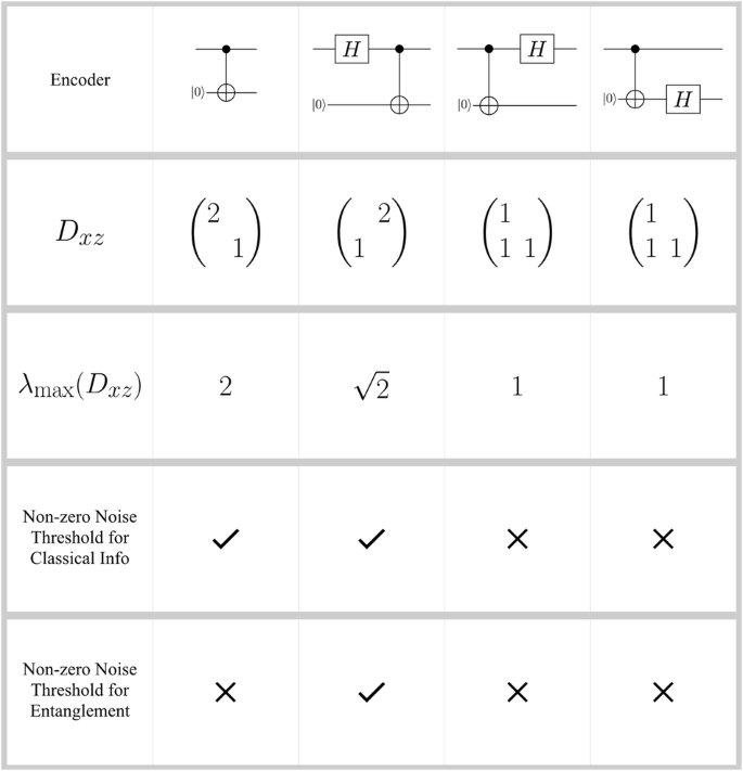
The encoder of the binary repetition code and 3 of its variations obtained by adding a single Hadamard gate to its inputs/outputs. In every circuit, the top qubit is the input data qubit and the bottom qubit is the ancilla initialized in state $\left\vert 0\right\rangle$. In addition to these 3 variations, there is a 4^th variation in which the Hadamard acts on the ancilla before applying the CNOT gate. However, in that case the encoder acts trivially on the input state. For each of these encoders, we indicate their weight transition matrix D_xz defined in Eq. (34) and its largest eigenvalue ${\lambda }_{\max }({D}_{xz})$. Furthermore, we indicate whether there exists a non-zero noise threshold below which the tree transmits classical information and/or entanglement to any depth. Eq. (35) puts an upper bound on the noise threshold for classical information in terms of ${\lambda }_{\max }({D}_{xz})$. In particular, for ${\lambda }_{\max }({D}_{xz})=1$ information does not propagate over the infinite tree; this is the case for the 3^rd and 4^th encoders. The second column, which is the encoder of the Bell tree in Fig. 2 yields a non-zero noise threshold for the propagation of classical information and entanglement on an infinite tree. It is worth noting that the transition matrix D_xz is not unique. For instance, for the third encoder one can choose Z_L = XI or Z_L = IZ. With X_L = ZX, the former choice yields ${\lambda }_{\max }({D}_{xz})=(1+\sqrt{5})/2$, whereas for the latter ${\lambda }_{\max }({D}_{xz})=1$; we pick the lower value for the tighter upperbound.

It is worth considering the two special cases of standard and anti-standard encoders of CSS codes. For standard encoders, there exist logical operators with

$$n(z\to z)={d}_{z},\,\,\,\,n(z\to x)=0$$

and

$$n(x\to x)={d}_{x},\,\,\,\,n(x\to z)=0,$$

which implies

$${\lambda }_{\max }({D}_{xz})=\frac{1}{2}\left({d}_{x}+{d}_{z}\right)+\frac{1}{2}| {d}_{x}-{d}_{z}| =\max \{{d}_{x},{d}_{z}\}.$$

(40)

Next, suppose we add a Hadamard to this encoder to obtain an anti-standard encoder with

$$n(z\to z)=0,\,\,\,\,n(z\to x)={d}_{x}$$

and

$$n(x\to x)=0,\,\,\,\,n(x\to z)={d}_{z},$$

which implies

$${\lambda }_{\max }({D}_{xz})=\sqrt{{d}_{x}\times {d}_{z}}.$$

(41)

Therefore, the bound in Eq. (36) generalizes the special bounds we have previously seen in the case of standard and anti-standard encoders.

Finally, we consider the most general stabilizer encoder which can be an arbitrary Clifford unitary. In this case, the logical σ_x and σ_z operators contain σ_x, σ_y, and σ_z. Then, in this situation, it is more natural to assume a noise model where X, Y, Z errors happen independently, each with probability p_x = p_y = p_z = p≤1/2. This corresponds to the depolarizing channel

$${{\mathcal{M}}}_{\epsilon }(\rho )={{\mathcal{N}}}_{x}\,{\circ}\, {{\mathcal{N}}}_{y}\,{\circ}\, {{\mathcal{N}}}_{z}(\rho )=(1-\epsilon )\rho +\epsilon \frac{I}{2},$$

(42)

where ϵ = 4p(1 − p), and ${{\mathcal{N}}}_{w}(\rho )=p{\sigma }_{w}\rho {\sigma }_{w}+(1-p)\rho$ for w = x, y, z.

Proposition 3

Let ${L}_{x},{L}_{y},{L}_{z}\in {\langle iI,{\sigma }_{x},{\sigma }_{y},{\sigma }_{z}\rangle }^{\otimes b}$ be logical σ_x, σ_y, and σ_z operators for the encoder $V:{{\mathbb{C}}}^{2}\to {({{\mathbb{C}}}^{2})}^{\otimes b}$, such that L_wV = Vσ_w: w = x, y, z. Let n(v → w) be the number of qubits on which logical σ_v acts as σ_w and consider the corresponding 3 × 3 matrix

$${D}_{xyz}=\left(\begin{array}{ccc}n(x\to x)&n(y\to x)&n(z\to x)\\ n(x\to y)&n(y\to y)&n(z\to y)\\ n(x\to z)&n(y\to z)&n(z\to z)\end{array}\right).$$

(43)

Let ${\lambda }_{\max }({D}_{xyz})$ be the spectral radius of D_xyz, i.e., the largest absolute value of the eigenvalues of D_xyz, and

$${b}_{\max }=\max \{{\rm{weight}}({L}_{x}),{\rm{weight}}({L}_{y}),{\rm{weight}}({L}_{z})\},$$

be the maximum weight of these logical operators. Assume the noise channel ${\mathcal{N}}$ that defines the tree channel ${{\mathcal{E}}}_{T}$ in Eq. (9) is the depolarizing channel ${{\mathcal{M}}}_{\epsilon }$ in Eq. (42). If

$$(1-\epsilon )\times \min \{{\lambda }_{\max }({D}_{xyz}),{b}_{\max }\} < 1,$$

(44)

then in the limit T → ∞, the output of channel ${{\mathcal{E}}}_{T}$ becomes independent of the input. More precisely, for any single-qubit density operator ρ, it holds that

$${\left\Vert {{\mathcal{E}}}_{T}(\rho )-{{\mathcal{E}}}_{T}\left(\frac{I}{2}\right)\right\Vert }_{1}\le 2\sqrt{2}\times \sqrt{{g}_{xyz}(T)\times {(1-\epsilon )}^{T}}.$$

(45)

Here,

$${g}_{xyz}(T)=\mathop{\max }\limits_{w\in \{x,y,z\}}\left(\begin{array}{ccc}1&1&1\end{array}\right){D}_{xyz}^{T}{e}_{w}\le {b}_{\max }^{T},$$

(46)

is an upper bound on the weights of logical operators in level T, where e_x = (1, 0, 0)^T, and e_y and e_z, are defined in a similar fashion.

To prove this result, we first show the following lemma, which is a generalization of proposition 1, and is of independent interest. Here, ${{\mathcal{D}}}_{w}$ is the single-qubit channel that fully dephases the input qubit in the eigenbasis of σ_w, i.e., ${{\mathcal{D}}}_{w}(\rho )=(\rho +{\sigma }_{w}\rho {\sigma }_{w})/2$.

Lemma 1

Let ${L}_{w}[T]\in {\langle iI,{\sigma }_{x},{\sigma }_{y},{\sigma }_{z}\rangle }^{\otimes {b}^{T}}$ be a logical σ_w operator, such that L_w[T]V_T = V_Tσ_w. Let ${\mathcal{N}}$ be the noise channel that defines the tree channel ${{\mathcal{E}}}_{T}$ in Eq. (9). Then,

$${\left\Vert {{\mathcal{E}}}_{T}-{{\mathcal{E}}}_{T}\,{\circ}\, {{\mathcal{D}}}_{w}\right\Vert }_{\diamond}^{2}\le 2\times r(T)\times {\rm{weight}}({L}_{w}[T]),$$

(47)

where

• (i) w = x, y, z and r(T) = (1−ϵ)^T, provided that ${\mathcal{N}}$ is the depolarizing channel ${{\mathcal{M}}}_{\epsilon }$ in Eq. (42).

• (ii) w = x, z, and r(T) = (1−2p)^2T, provided that ${\mathcal{N}}={{\mathcal{N}}}_{z}\,{\circ}\, {{\mathcal{N}}}_{x}$, with the probability of bit-flip and phase-flip errors p_x = p_z = p, and provided that there exists a sequence of operators L_w[0] → L_w[1] → ⋯ → L_w[T] such that L_w[0] = σ_w, ${L}_{w}[t]\in {\langle iI,{\sigma }_{x},{\sigma }_{z}\rangle }^{\otimes {b}^{t}}$, and ${L}_{w}[t+1]{V}^{\otimes {b}^{t}}={V}^{\otimes {b}^{t}}{L}_{w}[t]$ for all t ≥ 0.

In particular, in the first case of this lemma, if there exists a sequence of logical operators L_w[T] such that

$$\mathop{\lim }\limits_{T\to \infty }{(1-\epsilon )}^{T}\times {\rm{weight}}({L}_{w}[T])=0,$$

(48)

then the infinite tree is entanglement-breaking and might only transfer classical information encoded in the eigenbasis of σ_w. Note that this lemma does not assume the restriction that all encoders in the tree must be the same. Indeed, it can also be extended to stabilizer trees where the Clifford encoders are sampled randomly.

Comparison with bond percolation bound on noise threshold

The depolarizing channel ${{\mathcal{M}}}_{\epsilon }(\rho )=(1-\epsilon )\rho +\epsilon \frac{I}{2}$ has a simple probabilistic interpretation: it discards the input qubit with probability ϵ, and replaces it with the maximally mixed state. Therefore, in a quantum tree with this depolarizing noise channel on every edge, with probability ϵ, no information about the root is transmitted through each edge. This immediately allows us to apply the standard results from percolation theory¹², where each edge (or ‘bond’) of the tree is independently removed from the tree with probability ϵ. It is well-known that for a tree with branching number b, if (1 − ϵ) × b < 1, the probability of the existence of a continuous connected path from the root to the leaves in an infinite tree will approach zero^11,45. Note that the existence of such path from the root to leaves is only a necessary, but not a sufficient requirement for non-zero information propagation down to the leaves of a tree network.

We conclude that a quantum tree with depolarizing channel ${{\mathcal{M}}}_{\epsilon }$ on each edge will not transmit information to infinite depth when (1 − ϵ) × b < 1. Thus, the bond percolation threshold upperbound, i.e., 1 − 1/b, is an upperbound for the noise threshold for the propagation of information over infinite depth for any noisy quantum tree (not necessarily stabilizer trees), including trees where encoders are sampled randomly.

It is worth comparing this bound with the bound in Eq. (44), which is established for stabilizer trees: in general, $\min \{{\lambda }_{\max }({D}_{xyz}),{b}_{\max }\}\le b$. This means the latter bound will be stronger than the percolation bound (that is, it restricts the noise level ϵ that allows the transmission of information over infinite tree to a smaller range $\epsilon \le 1-1/\min \{{\lambda }_{\max }({D}_{xyz}),{b}_{\max }\}$).

Recursive decoding of trees with d ≥ 3 codes

In the previous section, we showed that above certain noise thresholds classical information and entanglement decay exponentially with depth T and vanish in the limit T → ∞. But, is there any non-zero noise level that allows the propagation of classical information and entanglement over the infinite tree? In this section, we answer in the affirmative by considering a simple recursive local decoding strategy for stabilizer trees with distance d ≥ 3.

We first explain the idea for general encoders and noise channels and then consider the special case of stabilizer codes with Pauli channels. Consider one layer of the tree channel, the channel ${{\mathcal{N}}}^{\otimes b}\,{\circ}\, {\mathcal{V}}$ that first encodes one input qubit in b qubits and then sends each qubit through the single-qubit noise channel ${\mathcal{N}}$. Let ${\mathcal{R}}:{\mathcal{L}}({({{\mathbb{C}}}^{2})}^{\otimes b})\to {\mathcal{L}}({{\mathbb{C}}}^{2})$ be a channel that (approximately) reverses this process, such that the concatenated channel $f[{\mathcal{N}}]={\mathcal{R}}\,{\circ}\, {{\mathcal{N}}}^{\otimes b}\,{\circ}\, {\mathcal{V}}$ is as close as possible to the identity channel (e.g., with respect to the diamond norm, or the entanglement fidelity), where for any single-qubit channel ${\mathcal{M}}$, we have defined

$$f[{\mathcal{M}}]\equiv {\mathcal{R}}\,{\circ}\, {{\mathcal{M}}}^{\otimes b}\,{\circ}\, {\mathcal{V}}.$$

(49)

As depicted in Fig. 6, by applying this recovery recursively, we find a recovery for the channel corresponding to the entire tree of depth T, denoted by ${{\mathcal{E}}}_{T}=\mathop{\prod }\nolimits_{j = 0}^{T-1}{{\mathcal{N}}}^{\otimes {b}^{j+1}}\,{\circ}\, {{\mathcal{V}}}^{\otimes {b}^{j}}$, or ${\widetilde{{\mathcal{E}}}}_{T}={{\mathcal{E}}}_{T}\,{\circ}\, {\mathcal{N}}$, if we consider the noise at the input qubit. Namely, the recovery is

$${{\mathcal{R}}}_{T}^{{\rm{loc}}}=\mathop{\prod }\limits_{i=0}^{T-1}{{\mathcal{R}}}^{\otimes {b}^{T-i-1}}.$$

(50)

As we will see in the following, in general, this is a sub-optimal recovery strategy. However, the advantage of this approach is that implementing the recovery does not require long-range interactions between distant qubits. More precisely, the error corrections are decided locally based on the observed syndromes from only one block with b qubits. Hence, we sometimes refer to this approach as local recovery, as opposed to the optimal recovery that would make a ‘global’ decision based on all observed syndromes together (see Sec. Optimal Decoding with Belief Propagation). Furthermore, as we discuss below, analyzing the performance of this recovery is relatively easy. We note that the recursive recovery approach has been previously studied in the context of concatenated codes with noiseless encoders³³ (in the language of this paper, this corresponds to the tree in which uncorrelated noise channels are applied to the qubits in the leaves, but not inside the tree).

Fig. 6: Derivation of the recursive equation (53).

After recovery upto level t, the effective noise channel is described by the single-qubit noise channel ${{\mathcal{N}}}_{t}$ defined in Eq. (51) (see the left image). In the middle image, we consider the single qubit channel obtained after applying recovery to a single block, i.e., $f[{{\mathcal{N}}}_{t}]={\mathcal{R}}\,{\circ}\, {{\mathcal{N}}}_{t}^{\otimes b}\,{\circ}\, {\mathcal{V}}$ (b = 2 in this diagram). In the right image, we compose this with the physical noise in the tree, i.e., ${{\mathcal{N}}}_{t+1}=f[{{\mathcal{N}}}_{t}]\,{\circ}\, {\mathcal{N}}$. Thus, the effective noise at the next level t + 1 is denoted by ${{\mathcal{N}}}_{t+1}$.

Fixed-point equation for infinite tree

For a tree with depth t, let ${{\mathcal{N}}}_{t}$ be the overall noise after applying the above recovery process to channel ${\widetilde{{\mathcal{E}}}}_{t}$, i.e.,

$${{\mathcal{N}}}_{\!t}={{\mathcal{R}}}_{t}^{{\rm{loc}}}\,{\circ}\, {\widetilde{{\mathcal{E}}}}_{t}={{\mathcal{R}}}_{t}^{{\rm{loc}}}\,{\circ}\, {{\mathcal{E}}}_{t}\,{\circ}\, {\mathcal{N}}.$$

(51)

As seen in Fig. 7, in a tree with depth t + 1 there are b subtrees each with depth t. For each subtree the effective error after error correction is ${{\mathcal{N}}}_{t}$. Then, ignoring the single-qubit channel ${\mathcal{N}}$ at the root of the tree with depth t + 1, the overall noise is

$$f({{\mathcal{N}}}_{\!t})={\mathcal{R}}\,{\circ}\, {{\mathcal{N}}}_{\!t}^{\otimes b}\,{\circ}\, {\mathcal{V}}.$$

(52)

Fig. 7: Recursive decoding of a tree.

This figure illustrates the steps of recursive decoding of a tree by indicating the subtree considered in each step. ${{\mathcal{N}}}_{t-1}$ and ${{\mathcal{N}}}_{t}$ are single-qubit channels obtained after the local recovery of subtrees of depth t − 1 and t, respectively. ${{\mathcal{N}}}_{t}$ can be expressed as a function of ${{\mathcal{N}}}_{t-1}$ and ${\mathcal{N}}$, as summarized in Eq. (53). This way of indexing local recovery levels will be followed in the rest of this paper.

Finally, adding the effect of the single-qubit channel ${\mathcal{N}}$ at the root, we obtain the overall noise channel

$${{\mathcal{N}}}_{t+1}=f({{\mathcal{N}}}_{t})\,{\circ}\, {\mathcal{N}}={\mathcal{R}}\,{\circ}\, {{\mathcal{N}}}_{t}^{\otimes b}\,{\circ}\, {\mathcal{V}}\,{\circ}\, {\mathcal{N}}.$$

(53)

Figure 6 illustrates Eq. (53). With the initial condition ${{\mathcal{N}}}_{0}={\mathcal{N}}$, this recursive equation fully determines ${{\mathcal{N}}}_{t}$ for arbitrary t. Then, in the limit t → ∞, we obtain the single-qubit channel

$${{\mathcal{N}}}_{\infty }=\mathop{\lim }\limits_{t\to \infty }{{\mathcal{N}}}_{t}=\mathop{\lim }\limits_{t\to \infty }{{\mathcal{R}}}_{t}^{{\rm{loc}}}\,{\circ}\, {\widetilde{{\mathcal{E}}}}_{t},$$

(54)

where we assume that the recovery channel is chosen properly such that this limit exists. This channel satisfies the fixed-point equation

$${{\mathcal{N}}}_{\infty }=f({{\mathcal{N}}}_{\infty })\,{\circ}\, {\mathcal{N}}={\mathcal{R}}\,{\circ}\, {{\mathcal{N}}}_{\infty }^{\otimes b}\,{\circ}\, {\mathcal{V}}\,{\circ}\, {\mathcal{N}}.$$

(55)

Note that the single-qubit channel ${{\mathcal{N}}}_{T}$ describes the output of the recursive recovery applied to the channel ${\widetilde{{\mathcal{E}}}}_{T}={{\mathcal{E}}}_{T}\,{\circ}\, {\mathcal{N}}$, which includes channel ${\mathcal{N}}$ at the input. On the other hand, if one does not include the single-qubit noise at the input of the tree, then the overall channel is described by $f({{\mathcal{N}}}_{T-1})$, and in the limit T → ∞, one obtains the channel $f({{\mathcal{N}}}_{\infty })$.

Depending on the strength of the noise in the single-qubit channel ${\mathcal{N}}$ and the properties of the encoder ${\mathcal{V}}$, the channel ${{\mathcal{N}}}_{\infty }$(or, $f({{\mathcal{N}}}_{\infty })$) might be a channel with constant output which does not transmit any information, i.e., with zero classical capacity, an entanglement-breaking channel with nonzero classical capacity, or a channel that transmits entanglement (and hence even classical information).

Recursive decoding of CSS code trees

In the following, we further study this approach for the case of CSS trees with standard encoders. In Supplementary Note D4 we explain how these results can be extended to general stabilizer trees.

We consider the recovery channel ${{\mathcal{R}}}_{T}^{{\rm{loc}}}$ defined in Eq. (50) applied to a CSS code tree ${\widetilde{{\mathcal{E}}}}_{T}$ which acts on X and Z errors separately. This ensures,

$${{\mathcal{R}}}_{T}^{{\rm{loc}}}\,{\circ}\, {\widetilde{{\mathcal{E}}}}_{T}={{\mathcal{Q}}}_{z}\,{\circ}\, {{\mathcal{Q}}}_{x}={{\mathcal{Q}}}_{x}\,{\circ}\, {{\mathcal{Q}}}_{z},$$

(56)

where ${{\mathcal{Q}}}_{z}={q}_{T}^{z}\rho +(1-{q}_{T}^{z})Z\rho Z$ is a phase flip channel, and ${{\mathcal{Q}}}_{x}={q}_{T}^{x}\rho +(1-{q}_{T}^{x})X\rho X$ is a bit flip channel. Since the cases of Z and X errors are similar, we focus on the recovery of Z errors and prove a lower bound on the noise threshold.

Proposition 4

Consider the tree channel ${\widetilde{{\mathcal{E}}}}_{T}={{\mathcal{E}}}_{T}\,{\circ}\, {\mathcal{N}}$ constructed from a standard encoder of a CSS code, as defined in Eq. (11). Suppose the single-qubit channel ${\mathcal{N}}={{\mathcal{N}}}_{z}\,{\circ}\, {{\mathcal{N}}}_{x}$ is composed of bit-flip and phase-flip channels ${{\mathcal{N}}}_{x}$ and ${{\mathcal{N}}}_{z}$ that apply X and Z errors with probabilities p_x and p_z, respectively. Suppose the minimum weight of the logical Z operator for this code is d_z, which means the code corrects up to t_z = ⌊(d_z − 1)/2⌋, Z errors. For sufficiently small probability of error p_z, e.g., for

$${p}_{z}\le \frac{{t}_{z}}{{t}_{z}+1}{\left(\frac{1}{({t}_{z}+1)c}\right)}^{\frac{1}{{t}_{z}}}\equiv \delta ,$$

(57)

the probability of logical Z error after local recovery is bounded by

$$\forall T:\,\,\,\,{q}_{T}^{z}\le \left(1+\frac{1}{{t}_{z}}\right){p}_{z},$$

(58)

where $c=\mathop{\sum }\nolimits_{k = {t}_{z}+1}^{b}\left(\begin{array}{c}b\\ k\end{array}\right)$ is a positive constant bounded as ${2}^{{t}_{z}}\le c\le {2}^{b}$. Furthermore,

$$\mathop{\lim }\limits_{{p}_{z}\to 0}\frac{{q}_{\infty }^{z}}{{p}_{z}}=1.$$

(59)

In particular, if t_z ≥ 1, then for p_z≤δ, the error ${q}_{T}^{z} < 1/2$, which means that the tree of any depth T transfers non-zero classical information in the input X basis. Thus, the logical single-qubit error in the infinite tree after local recovery is

$${q}_{\infty }^{z}\le \left(1+\frac{1}{{t}_{z}}\right){p}_{z}.$$

(60)

Also, note that ${q}_{T}^{z}$ is the probability of logical error in a tree with depth T with noise at the root (i.e., ${\widetilde{{\mathcal{E}}}}_{T}$). Clearly, without noise at the input channel, the overall noise is less. This proposition in proved in Methods Sec. Proof of Proposition 4. The general behavior of logical error after decoding is illustrated in Fig. 8.

Fig. 8: Summary of results for CSS code trees with distance d ≥ 3.

This plot illustrates the general behavior of the logical Z error ${q}_{T}^{z}$ in the channel ${\widetilde{{\mathcal{E}}}}_{T}={{\mathcal{E}}}_{T}\,{\circ}\, {\mathcal{N}}$, in the limit T → ∞ (i.e., the infinite tree with noise on the root) as a function of the physical Z error p on the edges of the tree. Here, d is the code distance, which in particular, means upto t_z = ⌊d_z − 1⌋/2 ≥ ⌊d − 1⌋/2, Z errors can be corrected. We characterize three regions, $p < \delta \equiv \frac{{t}_{z}}{1+{t}_{z}}{(\frac{1}{c(1+{t}_{z})})}^{\frac{1}{{t}_{z}}}$ (region I), $p > \frac{1}{2}(1-\frac{1}{\sqrt{d}})$ (region III), and the region in between (region II). From proposition 4 on local recovery analysis, we see that in region I, the logical error is bounded between p and $(1+{t}_{z}^{-1})\times p$, and it is $p+{\mathcal{O}}({p}^{2})$ for p ≪ 1. From our upperbound on the noise threshold, we see that in region III, the logical error in the infinite tree saturates to 1/2. The form of the curve in region II remains unknown, but it can be estimated for specific trees using the optimal recovery strategy in Sec. Optimal Decoding with Belief Propagation.

Recall that after recursive decoding, the effective single qubit channel is a concatenation of a bit-flip and phase-flip channel with error probabilities ${q}_{T}^{x}$ and ${q}_{T}^{z}$, respectively. As we explain in Supplementary Note B2, this channel is entanglement-breaking if, and only if, $| 1-{q}_{T}^{z}| \times | 1-{q}_{T}^{x}| < 1/2$. Proposition 4 ensures that we can make ${q}_{T}^{x}$ and ${q}_{T}^{z}$ arbitrarily small, by reducing p_x and p_z respectively. Therefore, there exists a non-zero value of p_x and p_z for which any infinite CSS code tree transmits entanglement.

Example: Noise threshold for recursive decoding of the repetition code tree

As a simple example, we consider the CSS code tree constructed from the standard encoder for the repetition code. Specifically, suppose the encoder at each node is

$$\left\vert c\right\rangle \,\longrightarrow \,V\left\vert c\right\rangle ={\left\vert c\right\rangle }_{L}={\left\vert c\right\rangle }^{\otimes b}\,\,\,:\,c\in \{0,1\},$$

(61)

for odd integer b. Classically the optimal error correction strategy for the repetition code can be realized via majority voting. In the quantum case measuring qubits in $\{\left\vert 0\right\rangle ,\left\vert 1\right\rangle \}$ basis and then performing majority voting destroys coherence between the logical states ${\left\vert 0\right\rangle }_{L}$ and ${\left\vert 1\right\rangle }_{L}$. However, one can perform majority voting in a way that does not destroy this coherence, namely by measuring stabilizers Z_jZ_j+1: j = 1, ⋯ , b − 1. Then, one determines the number of bit-flips (i.e., Pauli X) needed to make the eigenvalues of all stabilizers + 1. There are only two patterns of bit flips that make all the eigenvalues +1. Then, the decoder chooses the one that requires the minimum number of flips. We shall denote this b → 1 qubit recovery procedure with ${{\mathcal{R}}}_{{\rm{maj}}}$.

Assuming each qubit is subjected to independent bit-flip error, which flips the bit with probability p_x, the probability that the decoder makes a wrong guess is given by

$${\alpha }_{{\rm{maj}}}({p}_{x})=\mathop{\sum }\limits_{k=\lfloor b/2\rfloor +1}^{b}\left(\begin{array}{c}b\\ k\end{array}\right){p}_{x}^{k}{(1-{p}_{x})}^{b-k}.$$

(62)

We can compute the p_th as detailed in Methods Sec. Proof of Proposition 4. In particular, in Supplementary Note D we show that asymptotically in the limit of large b

$${p}_{{\rm{th}}}=\frac{1}{2}\left[1-\sqrt{\frac{\pi }{2}}\frac{1}{\sqrt{b}}\right]+{\mathcal{O}}\left(\frac{1}{b}\right).$$

(63)

On the other hand, applying the result of Evans et al.¹¹ on broadcasting over classical trees discussed in the introduction, we know that for the optimal recovery the exact threshold is

$${p}_{{\rm{th}}}^{{\rm{opt}}}=\frac{1}{2}\left[1-\frac{1}{\sqrt{b}}\right].$$

(64)

Interestingly, this threshold can also be achieved via similar majority voting, albeit when it is performed globally on all qubits at the output of the tree, whereas the threshold in Eq. (63) is obtained via recursive local majority voting on groups of b qubits. In Fig. 9 we compare the actual thresholds for the local and global majority voting approaches for finite values of b. See Supplementary Note E for further examples.

Fig. 9: Comparing the threshold for the recursive and optimal decoders.

Consider a full b-ary tree, where each node has the encoder $\left\vert c\right\rangle \mapsto {\left\vert c\right\rangle }^{\otimes b}:c=0,1$, for odd b. Also, assume each edge has a bit-flip channel, which applies Pauli X with probability p_x. The result of¹¹ implies that for the infinite tree, the noise threshold for transmission of classical information in the input Z basis is ${p}_{{\rm{th}}}^{{\rm{opt}}}=\frac{1}{2}(1-\frac{1}{\sqrt{b}})$. Meanwhile, applying the method described in the previous section to the function α_maj in Eq. (62), we numerically estimate the local recovery threshold p_th. The plot shows the ratio $(1-2{p}_{{\rm{th}}})/(1-2{p}_{{\rm{th}}}^{{\rm{opt}}})$. For large b, this ratio approaches $\sqrt{\pi /2}\approx 1.253$, matching the analytical result in Eq. (63).

Recursive Decoding of Trees with distance d = 2 codes

In this section, we consider trees where at each node the received qubit is encoded in a code with distance d = 2. Since such codes can not correct single-qubit errors in unknown locations, the local recovery approach discussed in the previous section fails to yield a non-zero threshold for infinite trees: under local recovery, the probability of logical error as a function of the probability of physical error has a linear term, which will then accumulate as the tree depth grows.

To overcome this issue, one may consider a modified version of the recursive recovery that combines several layers together and performs recovery on these combined layers, which corresponds to a concatenated code with distance d > 2. However, this modification will not solve the aforementioned issue because the noise between the layers still produces uncorrectable logical errors with a probability that is linear in the physical error probability.

To fix this problem, we introduce a new scheme, which takes advantage of the fact that although d = 2 codes cannot correct errors in unknown locations, they can (i) detect single-qubit errors, and (ii) correct single-qubit errors in known locations. Based on these observations, it is natural to consider a modification of local recovery where each layer sends a reliability bit to the next layer that determines if the decoded qubit is reliable or not. At each layer, the value of this bit is determined based on the value of the reliability bit received from the previous layers together with the syndromes observed in this layer. See Fig. 10 and Methods Sec. Recursive decoding with one reliability bit for further details.

Fig. 10: Recursive decoding with one reliability bit.

Figure a shows the decoding module for d = 2 codes with one reliability bit. It first applies the the unitary ${{\mathcal{U}}}^{\dagger }$, i.e., the inverse of encoder, on b input qubits ${\{{{\rm{q}}}_{i}(t-1)\}}_{i = 1}^{b}$, and then measures b − 1 ancilla qubits to obtain the syndromes ${\{{s}_{j}\}}_{j = 1}^{b-1}$. Then, it corrects the logical qubit with a unitary Corr controlled by the classical output of Algorithm 1 that classically processes ${\{{s}_{j}\}}_{j = 1}^{b-1}$ and ${\{{m}_{i}(t-1)\}}_{i = 1}^{b}$. The exact dictionary between the classical message+syndrome data and the correction unitary is determined by the encoding unitary ${\mathcal{U}}$. Furthermore, this algorithm also generates the reliability bit m(t) for the subsequent level t. Figure b presents the action of this decoder for T = 2 layers.

We rigorously prove and numerically demonstrate that using this recovery it is possible to achieve a noise threshold p_th strictly larger than zero for codes with distance d = 2. In particular, in Supplementary Note F we show that

Proposition 5

Consider the tree channel ${{\mathcal{E}}}_{T}$ defined in Eq. (9), for a b-ary tree of depth T. Suppose the noise at each edge is described by the Pauli channel

$${\mathcal{N}}(\rho )=(1-{p}_{{\rm{tot}}})\rho +{p}_{x}X\rho X+{p}_{y}Y\rho Y+{p}_{z}Z\rho Z,$$

where p_tot = p_x + p_y + p_z is the total probability of error. Assume the image of encoder $V:{{\mathbb{C}}}^{2}\to {({{\mathbb{C}}}^{2})}^{\otimes b}$ is a stabilizer error-correcting code [[b, 1, 2]], i.e., a code with distance 2. Then, for p_tot < 1/(16b⁴ + 4b²), after applying the recovery channel ${{\mathcal{R}}}_{T}$ in Methods Sec. Recursive decoding with one reliability bit, we obtain the Pauli channel

$${{\mathcal{R}}}_{T}\,{\circ}\, {{\mathcal{E}}}_{T}(\rho )=(1-{r}_{T}^{{\rm{tot}}})\rho +{r}_{T}^{x}X\rho X+{r}_{T}^{y}Y\rho Y+{r}_{T}^{z}Z\rho Z,$$

with the total probability of logical error ${r}_{T}^{{\rm{tot}}}={r}_{T}^{x}+{r}_{T}^{y}+{r}_{T}^{z}$, bounded by

$${r}_{T}^{{\rm{tot}}}\le (1+8{b}^{2})\times {p}_{{\rm{tot}}},$$

(65)

for all T.

Indeed, in Supplementary Note F we prove a slightly stronger result: recall that the final output of the recursive decoder in Fig. 10 is the decoded qubit along with the corresponding reliability bit m(T) whose value 1 indicates the likelihood of error in the decoded qubit (see Methods Sec. Recursive decoding with one reliability bit for further details). We show that if the total physical error is p_tot < 1/(16b⁴ + 4b²) then for all T the probability that the reliability bit m(T) = 1 remains bounded by 8b² × p_tot, and if m(T) = 0, then the probability of error on the decoded qubit is bounded by $(16{b}^{4}+4{b}^{2})\times {p}_{{\rm{tot}}}^{2}$, hence a quadratic suppression of undetected errors. Then, ignoring the value of the reliability bit m(T), the total probability of error is bounded as Eq. (65).

In conclusion, for p_tot < 1/(16b⁴ + 4b²), the probability of logical error ${r}_{T}^{{\rm{tot}}}$ is bounded by (1 + 8b²)/(16b⁴ + 4b²), even for the infinite tree. Since b ≥ 2, this means ${r}_{T}^{{\rm{tot}}}\le \sim 12 \%$, which implies that both classical information and entanglement propagate over the infinite tree (see Supplementary Note F).

As a simple example, in Fig. 11 we consider the tree constructed from the binary repetition encoder $\left\vert c\right\rangle \to \left\vert c\right\rangle \left\vert c\right\rangle \,:c=0,1$, with only bit-flip errors (p_z = p_y = 0). Note that technically this code has distance d = 1. Nevertheless, it detects single-qubit X errors, i.e., it has distance 2 for X errors. Our numerical analysis demonstrates the threshold is p_x ~ 0.125 which is consistent with the (albeit weak) lowerbound estimate from Proposition 5, ~ 0.3%. Note that in this case the exact threshold can be determined from the result of¹¹ on the classical broadcasting problem, namely Eq. (2) which implies ${p}_{{\rm{th}}}^{x}=(1-1/\sqrt{2})/2\approx 14 \%$.

Fig. 11: Performance of local recovery with one reliability bit on binary repetition code tree.

Suppose each node has the encoder of the binary repetition code, namely $\left\vert c\right\rangle \to \left\vert c\right\rangle \left\vert c\right\rangle :c=0,1$, and each edge has a bit-flip channel, which applies Pauli X with probability p_x. The decoder with one reliability bit achieves a non-zero noise threshold for information propagation in infinite trees: when p_x < ~ 0.125, the logical X error after local recovery of a tree with depth T → ∞ saturates to strictly below 0.5, while p_x > ~ 0.125 ensures the logical X error after recovery saturates to 0.5.

Finally, it is worth noting that for trees with standard or anti-standard encoders of CSS codes with distance 2 with independent X and Z errors on each edge, one can apply the recursive decoding strategy using two reliability bits – one for each type of error – to get improved performance.

Recursive decoding of Bell Tree (d = 1 code tree)

Next, we study the Bell tree, introduced in Fig. 2 in the introduction. Here, the encoder is an (anti-standard) encoder of the binary repetition code, which has distance d = 1: while it can detect a single X error (and correct none), it is fully insensitive to Z errors. Nevertheless, we show that if the probability of X and Z errors are sufficiently small (but non-zero) it is still possible to transmit both classical information and entanglement through the infinite tree. We show this using two different decoders: (i) the optimal decoder which is realized using a belief propagation algorithm discussed in the next section, and (ii) a sub-optimal decoder introduced in this section, which recursively applies a decoding module with two reliability bits (see Fig. 12).

Fig. 12: 2 levels of Bell tree and the corresponding recursive decoder.

${{\mathcal{R}}}_{Bell}$ is the decoder module described in Fig. 18. Each qubit is augmented with two reliability bits m^rel(t) and m^irrel(t), represented by double lines.

The relatively simple structure of this decoder makes it amenable to both analytical and numerical study. For instance, Fig. 13 presents the results of a numerical study of trees with depth up to T = 1000, which involves 2¹⁰⁰⁰ qubits. For this plot, the physical single-qubit noise in the tree channel ${{\mathcal{E}}}_{T}$ is ${\mathcal{N}}={{\mathcal{N}}}_{x}\,{\circ}\, {{\mathcal{N}}}_{z}$, where ${{\mathcal{N}}}_{x}$ and ${{\mathcal{N}}}_{z}$ are bit-flip and phase-flip channels, respectively, which apply X and Z errors, each with probability p_x = p_z = p. This numerical study shows that in the infinite tree for p < ~ 0.5% the probabilities of logical Z error ${q}_{\infty }^{z}$ and logical X error ${q}_{\infty }^{x}$ remain strictly smaller than 0.5; namely ${q}_{\infty }^{x}\le 7 \%$ and ${q}_{\infty }^{z}\le 3 \%$. This means that for p_x = p_z ≲ 0.5% both classical information and entanglement propagate to any depth in the Bell tree. Note that although the probability of physical X and Z errors are equal, the probability of logical errors ${q}_{T}^{x}$ and ${q}_{T}^{z}$ are not generally equal (see below for further discussion). In addition to these numerical results, in Supplementary Note G we also formally prove the existence of a non-zero threshold for this decoder, and estimate the noise threshold to be lowerbounded by ~ 0.245%, which is consistent with the numerical study. We describe this decoder that uses two reliability bits in Methods Sec. Recursive decoding of Bell Tree with two reliability bits. Furthermore, it is described more precisely in Algorithm 2 in Supplementary Note G, where we also present a rigorous error analysis for this algorithm.

Fig. 13: Performance of the recursive decoder with two reliability bits on the Bell trees.

We consider the Bell tree with depth T → ∞ with physical error p_x = p_z = p, ranging from 0.002 − 0.008 with step-size 0.001. These p values are shown on the corresponding colored curves, and p = 0.005 is highlighted. For p < ~ 0.005, the asymptotic logical X errors after decoding saturates to ${q}_{\infty }^{x}\le \sim 0.07$ (a similar result holds for ${q}_{\infty }^{z}$). On the other hand, for p > ~ 0.005 the asymptotic logical X and Z error saturate to 0.5.

We also note that the optimal decoder performance for T = 20 suggests that the actual threshold is lower than p_x = p_z ≈ 1.7%. It is also worth noting that the noise threshold for the decoder studied in this section is comparable with the actual noise threshold estimated by the optimal decoder (~0.5% versus ~1.7%), and the performance of the two decoders are similar in the very small noise regime, namely p_x = p_z ≪ 0.5%. Finally, recall that our results in Sec. CSS code trees with ‘Anti-standard’ encoders: Bell Tree imply exponential decay of information for p_x = p_z > (1 − 2^−1/4)/2 ≈ 8%.

Optimal decoding with belief propagation

Similar to any stabilizer code, the optimal decoding for the concatenated code defined by the tree encoder ${V}_{T}=\mathop{\prod }\nolimits_{j = 0}^{T-1}{V}^{\otimes {b}^{j}}$ can be performed by measuring the stabilizer generators. This can be realized by implementing the inverse of this encoder unitary and then measuring all the ancilla qubits in the Z basis. For a tree of depth T, this yields a syndrome bitstring s_T of length b^T − 1. In the absence of noise, one obtains the all-zero bit string and the remaining decoded qubit is equal to the input state of the tree. On the other hand, in the presence of an error, the output qubit is equal to the input, upto a logical error L_T = {I, X, Y, Z}. Then, any decoder uses the syndrome s_T to infer L_T and correct it by applying L_T on the decoded qubit. The optimal decoder needs to find L_T that maximizes the conditional probability p(L_T∣s_T). Prima facie, this would require an inefficient double-exponential search over ${2}^{{b}^{T}-1}$ distinct values of the syndromes.

However, thanks to the tree structure, it turns out that in the case that is of interest in this paper, the decoding can be performed exponentially more efficiently, in time ${\mathcal{O}}({2}^{T})$. In 2006, Poulin³⁴ developed an efficient algorithm for decoding concatenated codes via belief propagation (BP). This algorithm assumes the encoder is noiseless for the entire concatenated code and the qubits at the leaves of the tree are affected by Pauli errors that are uncorrelated between different qubits. On the other hand, errors between the encoders in the tree, that are considered in this paper, are equivalent to correlated errors on the leaves of the tree. Although the efficient algorithm of³⁴ cannot be extended to general correlated errors, as we explain below, it can be extended to the type of correlated errors that are caused by local errors in between encoders. Roughly speaking, this is possible because such correlations are consistent with the tree structure.

Belief propagation update rule

We explain how the algorithm works for the 3-ary tree of depth T = 2, presented in the example in Fig. 14. Each red dot in this figure corresponds to the Pauli noise channel

$${\mathcal{N}}(.)={r}_{I}(.)+{r}_{x}X(.)X+{r}_{y}Y(.)Y+{r}_{z}Z(.)Z.$$

To simplify the presentation, we have considered a tree with noise at the root.

Fig. 14: Optimal Decoding of a stabilizer tree.

The upper half of the figure is a tree with stabilizer encoder ${\mathcal{V}}$ along with Pauli noise ${\mathcal{N}}$ on each edge, which are denoted by red circles. The lower half is the application of the inverse unitaries U^† on the output of the tree process (Note that $V\left\vert \psi \right\rangle =U\left\vert \psi \right\rangle {\left\vert 0\right\rangle }^{\otimes (b-1)}$). Upon inversion, each ancillary qubit is measured in the Z-basis to obtain the syndromes. ${L}_{t}^{(i)}\in \{I,X,Y,Z\}$ indicates the overall logical error caused by the noise channels inside the dashed bubble above it, and ${s}_{t}^{(i)}$ is the corresponding syndrome string.

Recall that the optimal decoder needs to determine p(L_T∣s_T) for the observed value of s_T. Using the labeling introduced in Fig. 14. The goal is to determine

$$p\left({L}_{2}^{(1)}| {s}_{2}^{(1)},{s}_{1}^{(1)},{s}_{1}^{(2)},{s}_{1}^{(3)}\right).$$

Consider the action of the decoder circuit on the first level. Let error E be an arbitrary tensor product of Pauli operators and the identity operator. Then,

$${U}^{\dagger }EU={\mathcal{L}}(E)\otimes {{\bf{X}}}^{{\rm{Synd}}(E)}{{\bf{Z}}}^{{\bf{z}}},$$

(66)

where ${\mathcal{L}}(E)$ is the logical operator acting on the logical qubit and X^Synd(E) is the syndrome acting on the ancilla qubits. Since the ancilla is initially prepared in ${\left\vert 0\right\rangle }^{\otimes b-1}$, it remains unchanged under Z^z. We measure and record the syndrome Synd(E) in each step of decoding.

The key point is $p({L}_{2}^{(1)}| {s}_{2}^{(1)},{s}_{1}^{(1)},{s}_{1}^{(2)},{s}_{1}^{(3)})$ has a decomposition as

$$\begin{array}{l}p\left({L}_{2}^{(1)}| {s}_{2}^{(1)},{s}_{1}^{(1)},{s}_{1}^{(2)},{s}_{1}^{(3)}\right)\\ =\frac{1}{p({s}_{2}^{(1)}| {{\bf{s}}}_{1})}\sum _{{{\bf{L}}}_{1}}{f}_{{s}_{2}^{(1)}}\left({L}_{2}^{(1)},{{\bf{L}}}_{1}\right)\times \mathop{\prod }\limits_{i=1}^{3}p\left({L}_{1}^{(i)}| {s}_{1}^{(i)}\right),\end{array}$$

(67)

where ${{\bf{L}}}_{1}={L}_{1}^{(1)}{L}_{1}^{(2)}{L}_{1}^{(3)}$, ${{\bf{s}}}_{1}={s}_{1}^{(1)}{s}_{1}^{(2)}{s}_{1}^{(3)}$ and

$${f}_{{s}_{2}^{(1)}}\left({L}_{2}^{(1)},{{\bf{L}}}_{1}\right):= \delta \left[{s}_{2}^{(1)}={\rm{Synd}}({{\bf{L}}}_{1})\right]\times N\left({L}_{2}^{(1)}| {\mathcal{L}}({{\bf{L}}}_{1})\right),$$

where the conditional probability N describes the transition probability associated to Pauli channel ${\mathcal{N}}$, such that for any pair of E₁ and E₂ in the Pauli group,

$$N({E}_{1}| {E}_{2})={r}_{{E}_{1}{E}_{2}},$$

(68)

where E₁E₂ is the matrix product of Pauli operators E₁ and E₂ upto a global phase.

Notice that conditioned on ${s}_{1}^{(i)}$, the logical error ${L}_{1}^{(i)}$ is independent of the rest of the syndrome bits, which is clear from the tree structure. Now, this formula can be reapplied to $p({L}_{1}^{(i)}| {s}_{1}^{(i)})$ for each i. For instance, for the i = 1 subtree we have

$$p\left({L}_{1}^{(1)}| {s}_{1}^{(1)}\right)=\sum _{{{\bf{L}}}_{0}}{f}_{{s}_{1}^{(1)}}\left({L}_{1}^{(1)},{{\bf{L}}}_{0}\right)\frac{1}{p({s}_{1}^{(1)})}\times \mathop{\prod }\limits_{i=1}^{3}p\left({L}_{0}^{(i)}\right)$$

(69)

where ${{\bf{L}}}_{0}={L}_{0}^{(1)}{L}_{0}^{(2)}{L}_{0}^{(3)}$, and the superscript labels the three leaves in the first subtree. We can repeat this for the other two trees as well. At this point, we have reached level 0, i.e., the leaves of the tree. Therefore, when $p({L}_{0}^{(i)})$ appears in the expression, we have reached the terminal condition for recursion and we set $p({L}_{0}^{(i)})=N({L}_{0}^{(i)}| I)={r}_{{L}_{0}^{(i)}}$. See Supplementary Note H for further details of this algorithm for general stabilizer trees. In the following, we present some numerical examples.

Examples

Shor-9 Code – Fig. 15 plots the logical error for the tree as defined in Eq. (9) constructed from a Shor-9 code encoder that is standard in both X and Z. We consider trees of depths T = 1, 2, 3. The specifics of constructing this plot are explained in Supplementary Note H. We see that the asymptotic noise threshold for X errors is below ~ 0.17, whereas for Z errors it is below ~ 0.13 (since the number of Z stabilizers in the Shor-9 code is higher than X stabilizers and therefore this code is better equipped to correct X errors than Z errors). Recall that since this code has distance 3, our result in Proposition 1 establishes an upper bound ~ 0.21; thus, these numerics provide evidence for a tighter bound for the noise threshold.

Fig. 15: Optimal recovery of Shor-9 tree.

Probability of logical error as a function of the probability of physical error in the tree for trees of depth T = 1, 2 and 3. In plot a, the y-axis indicates the overall logical X-error after optimal decoding given the physical X noise within the tree has probability p_x indicated on the x-axis. Plot b shows the same quantities for Z errors. This provides improved upperbound estimates for noise threshold for X errors at ~ 0.17, and for Z errors at ~ 0.13. Each data point in the plots is computed via a Monte Carlo of 10⁵ samples explained in Supplementary Note H.

After optimal recovery for channel ${{\mathcal{E}}}_{T}$, the overall channel is a composition of a bit-flip and a phase-flip channel with the probability of X error and Z errors ${q}_{T}^{x},{q}_{T}^{z}\le 1/2$, respectively. Such channels are entanglement-breaking if, and only if, $| 1-{q}_{T}^{z}| \times | 1-{q}_{T}^{x}| < 1/2$ (see Supplementary Note B2). From numerical results in Fig. 15, it follows that for depth T = 3, this condition is satisfied for p > ~ 0.07. Note that since the error monotonically increases with T, the same also holds for T ≥ 3.

Steane-7 Code – Fig. 16 plots the optimal recovery performance for a tree as defined in Eq. (9) composed of Steane-7 encoders that are standard in both X and Z, and is similarly subject to independent X and Z errors for depths T = 1, 2, 3. Specifics of this recovery procedure are detailed in Supplementary Note H. Here, we see that the asymptotic noise threshold for X errors is below ~ 0.15. Because the Steane-7 code is self-dual, the same threshold holds true for the Z errors as well. Using an argument similar to the Shor-9 code, one can show that for p > ~ 0.07, entanglement cannot be transmitted beyond depth T ≥ 3.

Fig. 16: Optimal recovery of Steane-7 tree.

Probability of logical error as a function of the probability of physical error for trees of depth T = 1, 2, 3. Note that since Steane-7 code is self-dual X and Z errors have the same behavior, and therefore this plot presents both cases. In particular, x axis is the probability p_x = p_z of physical error in the channel. This provides upperbound estimates for asymptotic noise threshold for X (or, Z) error at p ~ 0.15. Each data point in the plots is computed via a Monte Carlo of 10⁵ samples explained in Supplementary Note H.

Mapping Quantum trees to classical trees with correlated errors

In this section, we argue that stabilizer trees can be understood in terms of an equivalent classical problem, which is a variant of the standard broadcasting problem on trees discussed in the introduction. For simplicity, we focus on trees constructed from a standard encoder of a CSS code with independent phase-flip and bit-flip channels.

Suppose we modify the original channel ${{\mathcal{E}}}_{T}$ defined in Eq. (9), by adding a fully dephasing channel ${{\mathcal{D}}}_{z}$ before and after each encoder. That is, at each node we modify the encoder ${\mathcal{V}}$ to

$${\mathcal{V}}\,\,\,\longrightarrow \,\,\,\overline{{\mathcal{V}}}\equiv {{\mathcal{D}}}_{z}^{\otimes b}\,{\circ}\, {\mathcal{V}}\,{\circ}\, {{\mathcal{D}}}_{z}.$$

(70)

Then, the channel ${{\mathcal{E}}}_{T}$ defined in Eq. (9) will be modified to

$${\overline{{\mathcal{E}}}}_{T}(\rho )=\mathop{\prod }\limits_{j=0}^{T-1}{\overline{{\mathcal{V}}}}^{\otimes {b}^{j}}\,{\circ}\, {{\mathcal{N}}}^{\otimes {b}^{j}}(\rho ),$$

(71)

which will be called the dephased tree in the following. Equivalently, rather than inserting dephasing channels ${{\mathcal{D}}}_{z}$, we can assume the probability of Z error p_z is increased to 1/2.

Then, at any level of the tree the density operator of qubits will be diagonal in the computational basis. In particular, the action of the dephased encoder $\overline{{\mathcal{V}}}$ is fully characterized by the classical channel with the conditional probability distribution

$${P}_{z}({\bf{z}}| c)=\left\langle {\bf{z}}\right\vert {\mathcal{V}}(\left\vert c\right\rangle \left\langle c\right\vert )\left\vert {\bf{z}}\right\rangle \,\,\,\,\,:\,c=0,1,{\bf{z}}\in {\{0,1\}}^{b}.$$

(72)

Note that the property that the density operator is diagonal in the computational basis remains valid under Pauli errors. In particular, Z errors act trivially on such states, whereas X errors, i.e., bit-flip channels, become a binary symmetric channel, which can described by the conditional probability

$${N}_{z}(j| i)={p}_{x}+(1-2{p}_{x}){\delta }_{i,j}\,\,\,:\,i,j=0,1.$$

(73)

Therefore, by adding dephasing before and after each encoder, as described in Eq. (70), we obtain a fully classical problem: at each node, a bit c ∈ {0, 1} enters the encoder, and at the output of the encoder a bit string z ∈ {0, 1}^b with probability P(z∣c) is generated. Then, each bit goes into a binary symmetric channel Q, which flips the input bit with probability p_x and leaves it unchanged with probability 1 − p_x. Finally, each bit goes to the next level and enters another encoder $\overline{{\mathcal{V}}}$.

The assumption that the encoder at each node is a standard encoder implies that the effect of inserted dephasing channels ${{\mathcal{D}}}_{z}$ in the middle of the tree is equivalent to correlated Z errors on the leaves. Furthermore, because for CSS codes Z and X errors can be corrected independently, we conclude that the probability of logical X error, ${q}_{T}^{x}$ for the dephased channel ${\overline{{\mathcal{E}}}}_{T}$ and the original channel ${{\mathcal{E}}}_{T}$ are equal. Another way to phrase this observation is to say that the distinguishability of the output states ${{\mathcal{E}}}_{T}(\left\vert 0\right\rangle \left\langle 0\right\vert )$ and ${{\mathcal{E}}}_{T}(\left\vert 1\right\rangle \left\langle 1\right\vert )$ with respect to any measure of distinguishability, such as the trace distance, is the same as the distinguishability of states ${\overline{{\mathcal{E}}}}_{T}(\left\vert 0\right\rangle \left\langle 0\right\vert )$ and ${\overline{{\mathcal{E}}}}_{T}(\left\vert 1\right\rangle \left\langle 1\right\vert )$. To prove this it suffices to show that there exists a channel ${{\mathcal{T}}}_{T}$ such that

$${{\mathcal{T}}}_{T}\,{\circ}\, {\overline{{\mathcal{E}}}}_{T}(\left\vert c\right\rangle \left\langle c\right\vert )={{\mathcal{E}}}_{T}(\left\vert c\right\rangle \left\langle c\right\vert )\,\,\,:c=0,1.$$

(74)

A channel ${{\mathcal{T}}}_{T}$ that satisfies the above equation is the error correction of Z errors, which requires measuring X stabilizers and correcting the Z errors based on the outcomes of the measurement, followed by adding certain (correlated) Z errors to reproduce the effect of Z errors in ${{\mathcal{E}}}_{T}$ (see proposition 6 in Supplementary Note I). Note that instead of the Z basis, we can dephase qubits in the X basis. This results in another classical tree with depth T, which can be used to determine the probability of logical Z error ${q}_{T}^{z}$. Similarly, in the case of CSS codes with anti-standard encoders the equivalent classical tree can be obtained by measuring the qubits in the Z and X bases, alternating between different levels (see the example below).

We conclude that any CSS tree with standard or anti-standard encoders and independent X and Z errors can be fully characterized in terms of a modification of the classical broadcasting problem which involves correlated noise on the edges that leave the same node. As an example, here we consider the classical tree corresponding to the Shor 9-qubit code. See Supplementary Note I2 for further examples.

Example: Bell tree

Consider the Bell tree discussed in Sec. Recursive Decoding of Bell Tree (d = 1 code tree) with noise rate p_x = p_z = p. Recall that the Bell encoder is an anti-standard encoder. Thus, as mentioned above, we must dephase alternatingly in the X and Z bases. Suppose we are interested in the propagation of information encoded in Z eigenstates (i.e., $\{\left\vert 0\right\rangle ,\left\vert 1\right\rangle \}$) of the input. Then, we shall dephase the root of the tree in the Z direction, then the next level must be dephased in the X direction, and so on. This implies that the dephased versions of two levels of a Bell tree is the concatenation of two kinds of classical encoders

$$\begin{array}{lll}{{\mathbb{M}}}_{1}\,:\,{P}_{z}(00| 0)=1\\\qquad\;\, {P}_{z}(11| 1)=1\end{array}$$

(75)

$$\begin{array}{lll}{{\mathbb{M}}}_{2}\,:\,{P}_{z}({\bf{w}}| 0)=1/2,{\rm{when}}\,{\bf{w}}\in \{00,11\}\\\qquad\;\,{P}_{z}({\bf{w}}| 1)=1/2,{\rm{when}}\,{\bf{w}}\in \{01,10\}\end{array}$$

(76)

that are present on alternate levels of the tree. For instance, the dephased version of a T = 2 Bell tree (as seen in Fig. 2) is,

$${{\mathbb{N}}}^{\otimes 4}\,{\circ}\, {{\mathbb{M}}}_{1}^{\otimes 2}\,{\circ}\, {{\mathbb{N}}}^{\otimes 2}\,{\circ}\, {{\mathbb{M}}}_{2},$$

(77)

where ${\mathbb{N}}$ represents the classical bit-flip channel that flips the input bit with probability p.

Discussion

This paper opens up several lines of inquiry. For instance, finding the exact noise threshold for the propagation of classical information and entanglement in an infinite tree remains an open question. A natural extension of this work is to consider other (non-Clifford) encoders and noise processes. In particular, the case of Haar-random (independent) unitaries^30,31 at different nodes is an interesting model for natural processes. Other noise models such as erasure noise or coherent noise can also be studied. While the current study assumes that the decoder has access to all the exponentially many qubits at the end of the tree, more pragmatically one can study how classical and quantum correlations are affected when we consider only a subset of the leaves instead of all of them. A thorough study of classical trees obtained by dephasing quantum trees (as explained in Supplementary Note I3) is an open question not just of independent interest within classical network theory, but with direct applications to CSS code trees. Finally, it would be interesting to further investigate the potential applications of the techniques introduced in this paper for understanding the so-called measurement-induced phase transition, which has been recently studied in condensed matter theory. In this context, qubits in an otherwise noiseless circuit are randomly measured, and a phase transition in the purity of the post-selected states is observed, depending on the probability of measurements (See, e.g.,^2,3,4,5 and^46,47 for networks with tree structure).

Methods

Proofs of Propositions 1, 2 and 3

Proofs of Propositions 1, 2, 3 and Lemma 1 are presented in Sec. Stabilizer Trees with Standard Encoders, CSS code trees with Standard Encoders, and CSS code trees with ‘Anti-standard’ encoders: Bell Tree, and are proved in Supplementary Notes C1 and C2.

Proof of Proposition 4

To analyze the performance of the local recursive strategy for a CSS code tree, we first note that for CSS codes with uncorrelated X and Z errors, error correction for these errors can be performed independently, and therefore after error correction, the X and Z errors remain uncorrelated. In particular, there exists a recovery process ${\mathcal{R}}$ that corrects X and Z errors independently, i.e., a recovery process ${\mathcal{R}}$ such that

$$f[{{\mathcal{M}}}^{x}\,{\circ}\, {{\mathcal{M}}}^{z}]=f[{{\mathcal{M}}}^{x}]\,{\circ}\, f[{{\mathcal{M}}}^{z}],$$

(78)

where ${{\mathcal{M}}}^{x}$ and ${{\mathcal{M}}}^{z}$ are bit-flip and phase-flip channels, respectively, and function f defined in Eq. (49) denotes the effective single-qubit channel after recovery. In particular, if ${{\mathcal{M}}}^{z}(\rho )=(1-p)\rho +pZ\rho Z$, then

$$f[{{\mathcal{M}}}^{z}](\rho )=(1-{\alpha }_{z}(p))\rho +{\alpha }_{z}(p)Z\rho Z,$$

(79)

where α_z(p) determines the probability of logical error after recovery. Note that α_z(1/2) = 1/2, which corresponds to the cases of maximal Z error. For instance, for the Steane-7 code

$${\alpha }_{z}(p)=21{p}^{2}-98{p}^{3}+210{p}^{4}-252{p}^{5}+168{p}^{6}-48{p}^{7}.$$

In Supplementary Note E we explain how this function can be calculated for general CSS codes (see also³³).

Now we consider the recursive Eq. (53) for the phase-flip channel ${{\mathcal{Q}}}_{z}$ in Eq. (56), which applies Z error with probability ${q}_{T}^{z}$. Writing Eq. (53) in terms of function α_z, we obtain

$${q}_{t+1}^{z}=(1-{p}_{z})\times {\alpha }_{z}({q}_{t}^{z})+{p}_{z}\times [1-{\alpha }_{z}({q}_{t}^{z})],$$

(80)

with the initial condition ${q}_{0}^{z}={p}_{z}$. The fixed point of this equation, denoted by ${q}_{\infty }^{z}$, satisfies

$${\alpha }_{z}({q}_{\infty }^{z})=\frac{{q}_{\infty }^{z}-{p}_{z}}{1-2{p}_{z}}.$$

(81)

Therefore, to determine ${q}_{\infty }^{z}$ we study the intersection of the curve α_z(q) with the line (q − p_z)/(1 − 2p_z) as functions of q (see Fig. 17). Since α_z(1/2) = 1/2, ${q}_{\infty }^{z}=1/2$ is always a solution. However, for a sufficiently small value of p_z, the two curves have more intersections in the interval $0 < {q}_{\infty }^{z} < 0.5$. Let ${p}_{{\rm{th}}}^{z}$ be the largest value of p_z for which they have an intersection in this interval. As it can be seen in Fig. 17 this point is determined by the tangent of curve α_z that passes through the point (0.5, 0.5). More specifically, ${p}_{{\rm{th}}}^{z}$ is the x-intercept for this line. Given α_z, ${p}_{{\rm{th}}}^{z}$ can be estimated numerically.

Fig. 17: Schematic for recursive decoding threshold computation.

Figure a shows the intersection of two curves α(q) and (q − p_z)/(1 − 2p_z), where p_z is the error within the tree and the line’s x-intercept. According to Eq. (81), for the infinite tree the overall error after the recovery, denoted by ${q}_{\infty }^{z}$, is determined by the the intersection of these two curves. The smallest x-value of the intersections is ${q}_{\infty }^{z}$. For large enough p_z, only the (0.5, 0.5) intersection persists, entailing that the infinite tree upon local recovery transmits no information. Figure b shows ${p}_{{\rm{th}}}^{z}$, i.e. the maximum value of p_z for which ${q}_{\infty }^{z}$ is not 0.5. Figure c shows that every α(q) for a [[b, 1, d]] CSS code is upper bounded by $c{q}^{\lfloor ({d}_{z}-1)/2\rfloor +1}$, for some constant ${2}^{{t}_{z}}\le c\le {2}^{b}$, where d_z ≥ d is the distance for Z errors. Consider the tangent line to this curve that passes the point (0.5, 0.5). The x-intercept of this tangent line is a lower bound on ${p}_{{\rm{th}}}^{z}$. Graphically, we see that this lowerbound is always greater than zero. Using this observation, in Supplementary Note D, we show that ${p}_{{\rm{th}}}^{z}$ is lower bounded by $\delta := \frac{{t}_{z}}{{t}_{z}+1}{\left(\frac{1}{({t}_{z}+1)c}\right)}^{\frac{1}{{t}_{z}}}$, which is strictly positive when d_z ≥ 3. We also show that for p_z less than this value, the logical error in the channel ${\widetilde{{\mathcal{E}}}}_{T}={{\mathcal{E}}}_{T}\,{\circ}\, {\mathcal{N}}$, is bounded by ${p}_{z}(1+\frac{1}{{t}_{z}})$.

While the exact threshold ${p}_{{\rm{th}}}^{z}$ depends on the detail of the polynomial α_z, its value is strictly positive, provided that the lowest order of q in polynomial α_z(q) is 2 or higher, which means the recovery corrects all single-qubit Z errors. This is always possible for codes with distance d ≥ 3. In particular, suppose the code distance for Z errors is d_z ≥ d, i.e., the code corrects Z errors with weight t_z = ⌊(d_z − 1)/2⌋ or less. Then, the lowest order of q in the polynomial α_z(q) is t_z + 1. Therefore, there exists a positive constant c, such that α_z(q) is upper bounded as

$${\alpha }_{z}(q)\le c\times {q}^{{t}_{z}+1},$$

(82)

where ${2}^{{t}_{z}}\le c\le {2}^{b}$ (see Supplementary Note D).

This, in turn, implies that the x-intercept of the tangent to $c{q}^{{t}_{z}+1}$ lower bounds the x-intercept of the tangent to α_z(q). Then, using an idea explained in Fig. 17, in Supplementary Note D we show that

$${p}_{{\rm{th}}}^{z}\ge \frac{{t}_{z}}{{t}_{z}+1}{\left(\frac{1}{({t}_{z}+1)c}\right)}^{\frac{1}{{t}_{z}}}\equiv \delta ,$$

(83)

thus, proving the first part of Proposition 4. Furthermore, from Fig. 17 it is clear that for ${p}_{z} < {p}_{{\rm{th}}}^{z}$ the overall probability of Z error in the infinite tree, denoted by ${q}_{\infty }^{z}$ can be arbitrarily small. In particular, we show that ${q}_{\infty }^{z}\le {p}_{z}\times (1+\frac{1}{{t}_{z}})$.

Finally, to show that $\mathop{\lim }\nolimits_{{p}_{z}\to 0}{q}_{\infty }^{z}/{p}_{z}=1$, consider the Taylor expansion of ${q}_{\infty }^{z}$ as a function of p_z in the limit p_z → 0, as ${q}_{\infty }^{z}={a}_{1}{p}_{z}+{\mathcal{O}}({p}_{z}^{2})$. Then, on the left-hand side of Eq. (81), the lowest degree of the polynomial ${\alpha }_{z}({q}_{\infty }^{z})$ in p_z is larger than or equal to 2, whereas on the right-hand side the lowest-degree term in p_z is (a₁ − 1) × p_z. Therefore, Eq. (81) implies a₁ = 1, hence $\mathop{\lim }\nolimits_{{p}_{z}\to 0}{q}_{\infty }^{z}/{p}_{z}=1$.

Proof of Proposition 5

We prove Proposition 5 in Supplementary Note F. We do so by performing a rigorous error analysis of the recursive decoding scheme that uses one reliability bit.

Recursive decoding with one reliability bit

Here, we present a full description of the recursive decoding with one reliability bit. Recall that at level t of recursive decoding of a tree of depth T, there are b^T−t identical blocks each with b qubits inside. Since noise affects all blocks in the same way and the same decoder is applied to all blocks, the following analysis applies to all the blocks at this level. Therefore, to simplify the notation, we suppress the indices that determine the block under consideration, and just label qubits inside a block with index i = 1, ⋯ , b. Let m_i(t − 1) be the corresponding reliability bits that are received from the previous level (see Fig. 10). In the following, we assume the reliability bit takes the value 1 when the qubit is unreliable or marked. For the first level of recovery, i.e., at the leaves of the tree, we assume the reliability bits are all initiated at 0.

Algorithm 1

Decoding module with one reliability bit

begin with b qubits i = 1, . . . , b and their corresponding reliability bits m_i(t − 1) received from level t − 1.

apply ${{\mathcal{U}}}^{\dagger }$ to the b qubits and measure the b − 1 ancilla qubits to obtain ${\{{s}_{j}\}}_{j}$

if m_i(t − 1) = 0, ∀ i then

 if s_j = 0, ∀ j then

 m(t) ← 0

else

 m(t) ← 1

end if

else if m_i(t − 1) = 1 for exactly one i ∈ {1, ⋯ , b}, denoted as k then

if s_j = 0, ∀ j then

 m(t) ← 0

else if some s_j ≠ 0, but ${\{{s}_{j}\}}_{j}$ are consistent with error on k^th qubit then

 correct logical qubit appropriately

 m(t) ← 0

else

 m(t) ← 1

end if

else

 m(t) ← 1

end if

return logical qubit and m(t) to t level.

Now, similar to the original local recovery in the previous section, the recovery starts by applying the inverse of the encoder circuit and then measuring b − 1 ancilla qubits, which determine the value of syndromes s_j : j = 1,..., b − 1. For codes with distance d = 2 this information is not enough to determine the location of the error. Therefore, unlike the original scheme, the Pauli correction applied to the logical qubit not only depends on these syndromes, but also depends on the value of reliability bits m_i(t − 1): i = 1,..., b. More specifically,

• 1. If no qubit is marked, i.e., m_i(t − 1) = 0 for i = 1, ⋯, b, and no syndrome is observed, i.e., s_j = 0 for all j = 1, ⋯, b − 1, then decode (without applying any correction) and set m(t) = 0, indicating the reliability of this qubit.

• 2. Similarly, if exactly one qubit is marked and no syndrome is observed then again decode and set m(t) = 0.

• 3. If exactly one qubit is marked and the observed syndromes are consistent with a single-qubit error in that location, then assume there is an error in that location, correct the error, and set m(t) = 0.

• 4. In all the other cases, decode ignoring the reliability bits and set m(t) = 1.

This procedure is also described more precisely in Algorithm 1. Two important remarks are in order here: First, note that only in case 3, the value of the reliability bits affect the applied correction. This is exactly where we take advantage of the fact that codes with distance 2 can correct single-qubit errors in a known location. Secondly, note that if all reliability bits m_i(t − 1) = 0: i = 1, ⋯ b and some error syndromes are observed, while the local recovery cannot correct the error, it sets m(t) = 1 signaling to the next layer that an error has been detected in this level. In this case, we take advantage of the error detection property of distance 2 codes.

Therefore, assuming the probability that a received qubit at this level has an error with probability p ≪ 1, the probability that the reliability bit is set to m(t) = 1 is of order b × p in the leading order. On the other hand, the probability of an undetected (and thus, unmarked) error is of order (b × p)². This suppression of the probability of error from order p to p², will make it possible to propagate information over an infinite tree, provided that the probability of physical noise in the single-qubit channels is sufficiently small.

Recursive decoding of Bell Tree with two reliability bits

Here, we present the full description of the recursive decoder with two reliability bits for the Bell tree. This procedure is described more precisely in Algorithm 2 in Supplementary Note G, where we also present a rigorous error analysis for this algorithm.

This decoder recursively applies the decoding module with the circuit diagram in Fig. 18. The example in Fig. 12 presents two layers of this decoder. Recall that at level t of recursive decoding of a Bell tree of depth T, there are 2^T−t identical blocks each with 2 qubits inside. Since the noise affects all the blocks in the same way and the same decoder is applied to all of them, similar to the previous section, we suppress the indices that determine the block under consideration and just label the two qubits inside a block with index i = 1, 2.

Fig. 18: Decoding module for the recursive decoder of the Bell tree.

This figure illustrates the three circuits involved in the Bell Tree decoding module from level t − 1 to t. The input to the module are two qubits q₁(t − 1) and q₂(t − 1) along with their ordered reliability bit pairs, labeled as ${\{({m}_{i}^{{\rm{rel}}}(t-1),{m}_{i}^{{\rm{irrel}}}(t-1))\}}_{i}$ for i = 1, 2. The first figure indicates the decoding circuit that detects the syndrome s and corrects the error based on ${m}_{i}^{{\rm{rel}}}(t-1):i=1,2$ and s. The bottom circuit generates the reliability bits sent to level t. It is segmented into relevant and irrelevant parts. The relevant part takes ${m}_{i}^{{\rm{rel}}}(t-1):i=1,2$and the syndrome s as the input, whereas the irrelevant part simply is an OR function on ${m}_{i}^{{\rm{irrel}}}(t-1):i=1,2$. Note that the `relevant' and `irrelevant' parts of the decoding module remain separate until the swapping of the bits at the end. This final swap accounts for the fact that the Bell encoder is an anti-standard encoder (see Sec. CSS code trees with `Anti-standard' encoders: Bell Tree).

Similar to Algorithm 1, here too the value of the reliability bits at each level is decided based on the observed syndrome and the reliability bits received from the previous level. Each reliability bit determines the likelihood of one type of error, namely X and Z errors, on the decoded qubit. At the first level (i.e., the leaves of the tree) all reliability bits are initiated at 0.

Consider the action of the decoding module in Fig. 18 on the leaves of the tree. The observed syndrome s is determined by the outcome of measuring Z ⊗ Z stabilizer on the pair of qubits in a block. On the other hand, since the decoding module applies a Hadamard gate on the decoded qubit, the measurement performed in the next level determines the outcome of X stabilizers measured on the leaf qubits. At each level, the decoding module should combine the information obtained from the syndrome measurement with the right type of reliability bits (X or Z). This can be achieved, e.g., by adding a third bit that keeps track of the parity of the current level, i.e., whether it is odd or even.

However, in the decoding module in Fig. 18, we use a slightly different approach that allows us to avoid the use of this additional bit. Namely, we keep this information in the order of the reliability bits: when qubits i = 1, 2 are received from the level t − 1, they each come with two reliability bits labeled as relevant and irrelevant bits. The relevant bit is determined by the values of the syndromes at levels t − 2, t − 4,..., which corresponds to the same type of stabilizer that is going to be measured at level t (i.e., X type or Z type).

More precisely, the decoding module in Fig. 18 is designed to realize the following rules:

• 1. Upon receiving qubits 1 and 2, measure the stabilizer Z₁ ⊗ Z₂ and denote the outcome by s.

• 2. For the pair of received qubits if both relevant reliability bits are zero, i.e., ${m}_{1}^{{\rm{rel}}}(t-1)\,{\rm{OR}}\,{m}_{2}^{{\rm{rel}}}(t-1)=0$, and no syndrome is observed (s = 0), then apply the inverse encoder without applying any correction and set the relevant reliability bit to zero, m^rel(t) = 0.

• 3. Similarly, if exactly one relevant reliability bit is 1, i.e., ${m}_{1}^{{\rm{rel}}}(t-1)\,{\rm{XOR}}\,{m}_{2}^{{\rm{rel}}}(t-1)=1$, and no syndrome is observed (s = 0), then apply the inverse encoder without applying any correction and set the relevant reliability bit to 0, i.e., m^rel(t) = 0.

• 4. If exactly one relevant reliability bit is 1 and the syndrome is observed (i.e., s = 1), then assume an error has happened on the marked qubit, correct the error, then apply the inverse encoder and set the relevant reliability bit to 0, i.e., m^rel(t) = 0.

• 5. In all the other cases, apply the inverse encoder ignoring the reliability bits and set m^rel(t) = 1.

• 6. Set the irrelevant reliability bit to 1 if any of the received irrelevant reliability bits are 1, i.e., ${m}^{{\rm{irrel}}}(t)={m}_{1}^{{\rm{irrel}}}(t-1)\,{\rm{OR}}\,{m}_{2}^{{\rm{irrel}}}(t-1)$, and then swap the relevant and irrelevant bits.

As mentioned, this procedure is described more precisely in Algorithm 2 in Supplementary Note G, where we also present a rigorous error analysis for this algorithm. It is worth noting that although the circuit in Fig. 18 implements the above rules, the order of implementation is slightly different: it first applies the inverse of the encoder and measures the ancilla qubit, and then applies the correction. It is also worth noting that only in case 4, a correction is performed, and after that the reliability bit is set to m^rel(t) = 0. It is interesting to consider a more “conservative” version of this decoder where in case 4, after the correction the relevant reliability bit is set to m^rel(t) = 1, indicating unreliability of the decoded qubit. Numerical results presented in Supplementary Note G suggests that this modification reduces the threshold to around ~ 0.3%, and generally results in a higher probability of logical error.

References

Preskill, J. Quantum Computing in the NISQ era and beyond. Quantum 2, 79 (2018).
Gullans, M. J. & Huse, D. A. Dynamical purification phase transition induced by quantum measurements. Phys. Rev. X 10, 041020 (2020).
Gullans, M. J. & Huse, D. A. Scalable probes of measurement-induced criticality. Phys. Rev. Lett. 125, 070606 (2020).
Skinner, B., Ruhman, J. & Nahum, A. Measurement-induced phase transitions in the dynamics of entanglement. Phys. Rev. X 9, 031009 (2019).
Li, Y., Chen, X. & Fisher, M. P. A. Measurement-driven entanglement transition in hybrid quantum circuits. Phys. Rev. B 100, 134306 (2019).
Von Neumann, J. Probabilistic logics and the synthesis of reliable organisms from unreliable components. Autom. Stud. 34, 43–98 (1956).
Pippenger, N. On networks of noisy gates. In 26th Annual Symposium on Foundations of Computer Science (sfcs 1985), 30–38 (IEEE, 1985).
Pippenger, N. Reliable computation by formulas in the presence of noise. IEEE Trans. Inf. Theory 34, 194–197 (1988).
Benjamini, I., Pemantle, R. & Peres, Y. Unpredictable paths and percolation. Ann. Probab. 26, 1198 – 1211 (1998).
Kesten, H. & Stigum, B. P. A limit theorem for multidimensional galton-watson processes. Ann. Math. Stat. 37, 1211–1223 (1966).
Evans, W., Kenyon, C., Peres, Y. & Schulman, L. J. Broadcasting on trees and the ising model. Ann. Appl. Probab. 10, 410–433 (2000).
Lyons, R. & Peres, Y. Probability on Trees and Networks, 42 of Cambridge Series in Statistical and Probabilistic Mathematics https://doi.org/10.1017/9781316672815 (Cambridge University Press, New York, 2016). Available at https://rdlyons.pages.iu.edu/
Mossel, E. Reconstruction on trees: Beating the second eigenvalue. Ann. Appl. Probab. 11, 285–300 (2001).
Mossel, E. & Peres, Y. Information flow on trees. Ann. Appl. Probab. 13, 817–844 (2003).
Wootters, W. K. & Zurek, W. H. A single quantum cannot be cloned. Nature 299, 802–803 (1982).
Barnum, H., Caves, C. M., Fuchs, C. A., Jozsa, R. & Schumacher, B. Noncommuting mixed states cannot be broadcast. Phys. Rev. Lett. 76, 2818–2821 (1996).
Google Quantum AI and Collaborators. Quantum error correction below the surface code threshold. Nature 638, 920–926 (2025).
Shor, P. W. Scheme for reducing decoherence in quantum computer memory. Phys. Rev. A 52, R2493–R2496 (1995).
Calderbank, A. R. & Shor, P. W. Good quantum error-correcting codes exist. Phys. Rev. A 54, 1098–1105 (1996).
Steane, A. M. Error correcting codes in quantum theory. Phys. Rev. Lett. 77, 793–797 (1996).
Gottesman, D.Stabilizer codes and quantum error correction. Ph.D. thesis https://login.proxy.lib.duke.edu/login?url=https://www.proquest.com/dissertations-theses/stabilizer-codes-quantum-error-correction/docview/304364982/se-2 (1997). Copyright - Database copyright ProQuest LLC; ProQuest does not claim copyright in the individual underlying works; Last updated - 2021-09-28.
Aharonov, D. & Ben-Or, M. Fault-tolerant quantum computation with constant error rate. SIAM Journal on Computing (2008).
Knill, E., Laflamme, R. & Zurek, W. Threshold accuracy for quantum computation. arXiv preprint quant-ph/9610011 (1996).
Gottesman, D. Fault-tolerant quantum computation with constant overhead (2014). 1310.2984.
Chamberland, C., Jochym-O’Connor, T. & Laflamme, R. Thresholds for universal concatenated quantum codes. Phys. Rev. Lett. 117, 010501 (2016).
Aharonov, D. Quantum to classical phase transition in noisy quantum computers. Phys. Rev. A 62, 062311 (2000).
Harrow, A. W. & Nielsen, M. A. Robustness of quantum gates in the presence of noise. Phys. Rev. A 68, 012308 (2003).
Razborov, A. A. An upper bound on the threshold quantum decoherence rate. Quantum Info Comput. 4, 222–228 (2004).
Kempe, J., Regev, O., Uunger, F. & de Wolf, R. Upper bounds on the noise threshold for fault-tolerant quantum computing. Quantum Info Comput. 10, 361–376 (2010).
Dalzell, A. M., Hunter-Jones, N. & Brandão, F. G. S. L. Random quantum circuits transform local noise into global white noise (2021). 2111.14907.
Deshpande, A. et al. Tight bounds on the convergence of noisy random circuits to the uniform distribution (2022). 2112.00716.
Dalzell, A. M., Hunter-Jones, N. & Brandão, F. G. S. L. Random quantum circuits anticoncentrate in log depth. PRX Quantum 3, 010333 (2022).
Rahn, B., Doherty, A. C. & Mabuchi, H. Exact performance of concatenated quantum codes. Phys. Rev. A 66, 032304 (2002).
Poulin, D. Optimal and efficient decoding of concatenated quantum block codes. Phys. Rev. A 74, 052333 (2006).
Shi, Y.-Y., Duan, L.-M. & Vidal, G. Classical simulation of quantum many-body systems with a tree tensor network. Phys. Rev. A 74, 022320 (2006).
Barthel, T., Lu, J. & Friesecke, G. On the closedness and geometry of tensor network state sets. Lett. Math. Phys. 112, 72 (2022).
Giovannetti, V., Lloyd, S. & Maccone, L. Quantum random access memory. Phys. Rev. Lett. 100, 160501 (2008).
Giovannetti, V., Lloyd, S. & Maccone, L. Architectures for a quantum random access memory. Phys. Rev. A 78, 052310 (2008).
Roberts, D. A. & Stanford, D. On memory in exponentially expanding spaces. J. High. Energy Phys. 2013, 1–26 (2013).
Almheiri, A., Dong, X. & Harlow, D. Bulk locality and quantum error correction in ads/cft. J. High. Energy Phys. 2015, 1–34 (2015).
Pastawski, F., Yoshida, B., Harlow, D. & Preskill, J. Holographic quantum error-correcting codes: Toy models for the bulk/boundary correspondence. J. High. Energy Phys. 2015, 1–55 (2015).
Nielsen, M. A. & Chuang, I. Quantum computation and quantum information. Am. J. Phys. 70, 558–559 (2002).
Calderbank, A. R., Rains, E. M., Shor, P. W. & Sloane, N. J. A. Quantum error correction and orthogonal geometry. Phys. Rev. Lett. 78, 405–408 (1997).
Helstrom, C. W. Quantum detection and estimation theory. J. Stat. Phys. 1, 231–252 (1969).
Evans, W. S. & Schulman, L. J. Signal propagation and noisy circuits. IEEE Trans. Inf. Theory 45, 2367–2373 (1999).
Feng, X., Skinner, B. & Nahum, A. Measurement-induced phase transitions on dynamical quantum trees. PRX Quantum 4, 030333 (2023).
Ferté, B. & Cao, X. Quantum darwinism-encoding transitions on expanding trees. Phys. Rev. A 109, 032226 (2024).
Acknowledgements
This work is supported by a collaboration between the US DOE and other Agencies. This material is based upon work supported by the U.S. Department of Energy, Office of Science, National Quantum Information Science Research Centers, Quantum Systems Accelerator. Additional support is acknowledged from NSF QLCI grant OMA-2120757, NSF grant FET-1910571, NSF FET-2106448. We acknowledge helpful discussions with Thomas Barthel, Ken Brown, Daniel Gottesman, Michael Gullans, David Huse, Jianfeng Lu, Henry Pfister, and Grace Sommers. SAY sincerely thanks Saathwik Yadavalli for all the time and effort he volunteered for making figures for the paper despite his busy schedule.
Author information
Authors and Affiliations
Contributions
S.A.Y. and I.M. contributed equally to this work.
Corresponding authors
Ethics declarations
Competing interests
The authors declare no competing interests.
Additional information
Publisher’s note Springer Nature remains neutral with regard to jurisdictional claims in published maps and institutional affiliations.
Supplementary information
Rights and permissions
Open Access This article is licensed under a Creative Commons Attribution-NonCommercial-NoDerivatives 4.0 International License, which permits any non-commercial use, sharing, distribution and reproduction in any medium or format, as long as you give appropriate credit to the original author(s) and the source, provide a link to the Creative Commons licence, and indicate if you modified the licensed material. You do not have permission under this licence to share adapted material derived from this article or parts of it. The images or other third party material in this article are included in the article’s Creative Commons licence, unless indicated otherwise in a credit line to the material. If material is not included in the article’s Creative Commons licence and your intended use is not permitted by statutory regulation or exceeds the permitted use, you will need to obtain permission directly from the copyright holder. To view a copy of this licence, visit http://creativecommons.org/licenses/by-nc-nd/4.0/.
About this article
Cite this article
Yadavalli, S.A., Marvian, I. Noisy quantum trees: infinite protection without correction. npj Quantum Inf 11, 151 (2025). https://doi.org/10.1038/s41534-025-00961-x
Received:
Accepted:
Published:
Version of record:
DOI: https://doi.org/10.1038/s41534-025-00961-x