
Abstract
This study introduces population history learning by averaging sampled histories (PHLASH), a new method for inferring population history from whole-genome sequence data. It works by drawing random, low-dimensional projections of the coalescent intensity function from the posterior distribution of a pairwise sequentially Markovian coalescent-like model and averaging them together to form an accurate and adaptive estimator. On simulated data, PHLASH tends to be faster and have lower error than several competing methods, including SMC++, MSMC2 and FITCOAL. Moreover, it provides automatic uncertainty quantification and leads to new Bayesian testing procedures for detecting population structure and ancient bottlenecks. The key technical advance is a new algorithm for computing the score function (gradient of the log likelihood) of a coalescent hidden Markov model, which has the same computational cost as evaluating the log likelihood. PHLASH has been released as an easy-to-use Python software package and leverages graphics processing unit acceleration when available.
Main
Many natural populations experience substantial changes in abundance over the course of their existence. Our species, for example, has increased over a 1,000-fold since the advent of agriculture around 12,000 years ago, with various human subpopulations having expanded or contracted due to migration, disease, climate change, interbreeding and other factors1,2,3,4. Generally, while some shifts may be attributable to random chance, measurable growth and decline over evolutionary timescales are frequently the result of interesting biological, cultural or ecological phenomena. By developing tools to estimate population history from genetic data, a pursuit known as demographic inference, we may hope to learn more about the past and possible future of our biome.
That said, estimating population history can be lamentably difficult. Signals of this history are only faintly manifested as patterns of allele sharing across sampled individuals. These patterns can be further obscured by natural phenomena such as meiotic recombination or natural selection, or by bioinformatic error. Complex mathematical models are needed to relate the data to a hypothesized size history. Solving these models is computationally expensive, particularly when a large number of samples is analyzed. Moreover, because of a somewhat diffuse relationship between the model and the data, there can be many evolutionary histories that explain a given collection of observations equally well5,6,7.
Nevertheless, given the potential to enhance our understanding of evolution, substantial effort has been invested in developing accurate and user-friendly methods for inferring population size history. An early and well-known example is the pairwise sequentially Markovian coalescent (PSMC)8, which infers a historically adequate population size using data from a single diploid individual. PSMC works by relating local variation in ancestry between pairs of chromosomes to fluctuations in historical population size. PSMC is fast, relatively robust and does not require phased genotypes, which can be challenging to obtain when working with nonhuman data9,10. However, PSMC is not without limitations: as originally formulated, the method can only analyze data from a single sample, and it assumes a fairly simplistic evolutionary model in which size history changes at only a small number of predetermined locations. The latter property leads to obvious visual bias in the resulting estimates, which have a ‘stair-step’ appearance, and has other, more obscure consequences for inference as well11,12.
A number of successor methods have been proposed, which remove some of these limitations13,14,15,16,17. Building on the basic PSMC model, they can analyze larger sample sizes and/or more realistic demographic models involving, for example, population structure and admixture. Several Bayesian variants of PSMC have also been proposed12,18,19, although they are not as widely used, owing perhaps to the inherent computational difficulty of Bayesian inference in this setting. Also, a large related class of methods exists that infer demography using the site frequency spectrum (SFS), a highly compressed summary statistic formed from genotype data20,21,22,23,24,25,26,27,28. These methods are fast, in some cases capable of analyzing tens of thousands of samples, but they ignore linkage disequilibrium (LD) information, which contains rich information about population history.
This study presents population history learning by averaging sampled histories (PHLASH), a new Bayesian method for inferring size history from recombining sequence data. PHLASH aims to combine the advantages of many of the methods mentioned above into a single, general-purpose inference procedure that is simultaneously fast, accurate, able to analyze many samples (thousands), invariant to phasing, capable of using both linkage and frequency spectrum information and able to return a full posterior distribution over the inferred size history function. Esthetically, PHLASH estimates have an appealing nonparametric quality that lets them adapt to variability in the underlying size history without user intervention or fine-tuning. The key advance that propels these innovations is a new technique for efficiently differentiating the PSMC likelihood function, which enables the method to navigate to areas of high posterior density more effectively. Combined with a highly efficient, graphics processing unit (GPU)-based software implementation, the end result is a method for performing full Bayesian inference of population size history at speeds that can exceed many of the optimized methods surveyed above.
Results
A typical output from PHLASH compared to other inference methods is shown in Fig. 1. For most applications, the main quantities of interest will be the posterior median of the sampled size histories (Fig. 1, dark blue lines). As shown below, the posterior median has good accuracy as a point estimator. PHLASH also quantifies uncertainty by a full posterior distribution over size histories (Fig. 1, right). For example, in Fig. 1, the posterior becomes more dispersed for t < 103, because there are not as many recent coalescent events available to accurately estimate ne.

Left: a number of (n = 100) diploid samples were simulated according to the size history shown via black line14,29. The posterior distribution returned by PHLASH is summarized by its median (dark blue line), and credible intervals are also returned. Right: the raw output from PHLASH, an ensemble of piecewise constant demographic histories, is also shown.
Accuracy compared to existing methods
PHLASH was first evaluated on simulated data where the ground truth is known. Its performance was then compared to that of the following three existing methods: SMC++, MSMC2 and FITCOAL. SMC++15 is a generalization of PSMC, which also incorporates frequency spectrum information by modeling the expected SFS conditional on knowing the TMRCA of a pair of distinguished lineages. MSMC2 (ref. 17) optimizes a composite objective where the PSMC likelihood is evaluated over all pairs of haplotypes. Finally, FITCOAL28 is a newer method that uses the SFS to estimate size history. These methods were chosen because they are relatively recent, have an easy-to-use software implementation, and can run on nonhuman data (that is, do not require phased data or detailed genetic maps).
The methods were compared across a panel of 12 different demographic models from the stdpopsim catalog29. Each model is the result of a previously published study. A key objective of PHLASH is to ensure its general applicability across a broad spectrum of biological systems. To that end, a total of eight different species are represented in the benchmark suite—Anopheles gambiae, Arabidopsis thaliana, Bos taurus, Drosophila melanogaster, Homo sapiens, Pan troglodytes, Papio anubis and Pongo abelii. Additional details of each model are shown in Supplementary Table 1.
To perform the benchmarks, whole-genome data were simulated under each of the models for diploid sample sizes n ∈ {1, 10, 100}. Three independent replicates were performed, resulting in a total of 12 × 3 × 3 = 108 different simulation runs. For some species, such as A. gambiae, the population-scaled recombination rate is so high that the default simulation engine for stdpopsim30 did not terminate after 24 h. Thus, for uniformity, all simulations were performed using the coalescent simulator SCRM31.
Each inference method was run on each of the simulated datasets. All methods were limited to 24 h of wall time and 256 GB of RAM. This meant that it was only possible to run some of the methods for certain sample sizes—SMC++ could only analyze n ∈ {1, 10} in the allotted amount of time, MSMC2 could only analyze n ∈ {1, 10} in the allotted amount of memory and FITCOAL could only analyze n ∈ {10, 100} in the allotted amount of time (it crashed with an error for n = 1). The command lines used for simulation and estimation are listed in Supplementary Note—Command lines—and summarized plots of every model fit are provided in Supplementary Figs. 6–9.
Three accuracy metrics were considered. The first metric, root mean-squared (or L2) error, has previously been used to compare the accuracy of demographic inference methods32,33. Root mean square error (RMSE) is defined here as
where n0(t) is the true historical effective population size that was used to simulate data, and T is an arbitrarily chosen time cutoff; the parameter T was set to 106 generations. This measure corresponds to the squared area between two population curves when plotted on a log–log scale, a common practice in population genetics. Compared to integration on a linear scale, it places greater emphasis on accuracy in the recent past and accuracy for smaller values of ne.
Results are shown in Extended Data Table 1. No method uniformly dominates, but overall, PHLASH tended to be the most accurate most often and is competitive with the most accurate method even when it is not—PHLASH achieved the highest accuracy in 22 of the 36 scenarios considered (61%), compared with 4 of 36 for FITCOAL, 5 of 36 for SMC++ and 5 of 36 for MSMC2. For n = 1 scenario, where only a single diploid genome is available, the difference in performance between PHLASH and SMC++/MSMC2 tended to be small and sometimes in favor of the latter methods. This is attributed to the nonparametric nature of the PHLASH estimator, which does not benefit from substantial prior regularization and generally requires more data to perform well. Also, as can be seen for the Constant model, FITCOAL is extremely accurate when the true underlying model is a member of its assumed model class, that is, consisting of a small number of epochs of constant or exponential growth. However, it is not clear that this is a reasonable assumption for natural populations; indeed, the real data results presented below seem to suggest otherwise.
Although RMSE is a common error metric, it does not necessarily paint a complete picture, because portions of the size history function may be effectively inestimable by any method due to the coalescent sampling process. This can happen, for example, when estimating very recent population history in an exponentially growing population or very ancient history in a population that has undergone a bottleneck. In both cases, the lack of coalescent events renders these time periods ‘invisible’ to coalescent-based demographic inference methods6,34. In these time periods, L2 error represents algorithm bias only because there is minimal signal to guide the estimator. Because, ultimately, size history inference is a density estimation problem, a natural alternative measure is the total variation (TV) distance between inferred and true demographic models. TV distance is bounded between zero and one and can be interpreted as the percentage difference between the underlying coalescent density functions (Supplementary Note—Total variation distance). Results for TV are shown in Extended Data Table 2. When considering TV error, PHLASH was most accurate two-thirds of the time (24/36 scenarios).
Finally, the ability of each method to match the empirically observed allele frequency spectrum was considered. Extended Data Table 3 shows the TV distance between the observed and fitted frequency spectra averaged over simulation replicates. Of note, n = 1 is not considered here because the frequency spectrum is degenerate in this case. PHLASH produced the closest match in 15 of 24 scenarios considered. This is noteworthy because two of the other methods, SMC++ and FITCOAL, also use frequency spectrum information; in the latter case, it is the only statistic that is matched to the data. It is conjectured that PHLASH performs better because it makes fewer assumptions about the underlying model class, providing greater flexibility to fit the observed frequency spectrum.
Running time and memory consumption
Next, the computational resources required by each method were examined. The peak amount of memory used, as well as total central processing unit (CPU) time, was recorded for each simulation run. Because the datasets were simulated from organisms with differing genome lengths, both measures were normalized by genome length (measured in gigabase (Gb) pairs) to enable comparison across runs, and the data from all runs were then averaged for each method and sample size.
The benchmarking results (CPU time and memory usage) described in the preceding paragraph are shown in Fig. 2. For analyzing a single diploid sample, n = 1, all methods required a similar amount of CPU time, around 20–30 min Gb−1; MSMC2 required the most memory, and PHLASH required the least. For n = 10, the only sample size where it was possible to run all four methods, FITCOAL was the most efficient in terms of time and memory usage, which was expected because it only analyzes the frequency spectrum. Of the hidden Markov model (HMM)-based approaches, PHLASH required substantially less CPU time and memory than SMC++ and, especially, MSMC2. Increasing the sample size to n = 100 caused the running time of FITCOAL to increase by roughly tenfold, while memory consumption remained low; for PHLASH, CPU and memory demands increased only moderately. Finally, for n = 1,000, no method except PHLASH was able to run given the allotted computational resources, and analyzing it required roughly the same amount of memory and less CPU time than analyzing ten samples using MSMC2.

For each method, the average was taken across 12 models × 3 replicates = 36 simulated datasets. Error bars represent mean ± 1 s.e.
Additional analyses
The Supplementary Note details the additional experiments conducted to evaluate the robustness of PHLASH under varying model conditions. Supplementary Note—Accuracy of the parallel approximation—verifies that the method used for parallelizing the computation of the log likelihood (Supplementary Note—Parallel evaluation) does not introduce too much error. Similarly, Supplementary Note—Calibration of the composite likelihood posterior—checks that the composite likelihood approximation (see Methods) does not cause the posterior distribution to become overconfident. Finally, Supplementary Note—Inferring recombination rates—investigates recombination rate inference.
Applications
Having verified that PHLASH performed well on simulated examples, the analysis was extended to real data. The analyses in this section are based on a recently published unified genomes dataset generated in ref. 35. The dataset contains 3,601 modern samples, as well as several archaic samples, obtained from a variety of sources36,37,38,39,40,41. The samples are organized into 214 different subpopulations; however, there is some duplication among them—for example, Human Genome Diversity Project (HGDP), Simons Genome Diversity Project and 1,000 Genomes Project all contain samples from the Yoruba population. After merging samples from duplicated populations, 159 populations remained; all of the descriptors below refer to the data after merging. Except where noted, all of the estimates assume a human mutation rate of 1.29 × 10⁻⁸ per base pair per generation and a generation time (g) of 29 years.
Inferring demographic history
The main use of PHLASH is to infer population history. Figure 3a shows the results of running PHLASH on all 159 populations in the dataset. For clarity, the populations were grouped into six geographical superpopulations, with an additional group for the archaic samples, and PHLASH was run on the combined data. The estimates recover some of the known motifs of human evolution, including shared ancestry in the ancient past, the African/non-African divergence about 3,500 generations ago, recent rapid expansion, a deep divergence between the African and non-African lineages, divergence of the Oceania super-population from a Eurasian ancestral population42 and the gradual extinction of the archaic populations.
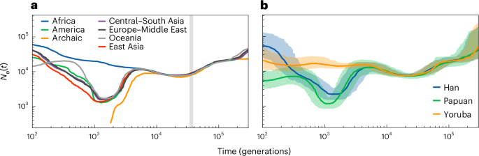
a, The estimates for modern populations. The vertical shaded region is 813–930 kya (see ‘Detecting a population bottleneck’). b, Estimates for specific populations considered in ‘Detecting a population bottleneck’, with shaded areas showing 95% credible interval.
PHLASH outputs more than just point estimates—Fig. 3b visualizes the posterior distribution for the Han, Yoruba and Papuan subpopulations. The width of the confidence bands can address more nuanced questions about how the populations evolved—they show, for example, increased uncertainty in the ancient as well as very recent past. Another interesting feature concerns population divergence. While Fig. 3a shows the African/non-African divergence occurring approximately 3,500 generations ago, Fig. 3b reminds us that the estimates are noisy; a reasonable lower bound on the divergence time could be when the Yoruba and Han/Papuan credible bands diverge, roughly 2,000 generations ago, or ~72 kya assuming a generation time of 29 years.
Detecting population structure
Given data from multiple populations, it is often of interest to understand when those populations diverged and whether they continue to exchange genetic material14. A useful statistic for this purpose, called the cross-coalescent rate (CCR), was defined in ref. 14. The CCR is 2η12/(η11 + η22), where ηij denotes the instantaneous rate of coalescence between a haplotype sampled from population i and one sampled from population j. CCR curves have been used as a model-free way of detecting population divergence and admixture9,17.
However, estimating η12 requires accurately phased data, which may be difficult to obtain in practice. A ‘nonphased’ analog of η12 can be formed by pooling samples from both populations and then estimating the coalescent intensity function on the pooled data, resulting in the statistic 2ηcombined/(η1 + η2). To investigate this idea, data from the Yoruba, Han, and European populations were analyzed. Results are shown in Fig. 4, with data generated according to a previously published out-of-Africa model20. In this model, basal CEU/CHB population diverges from YRI around 6,500 generations ago, with residual gene flow until the present (CEU, CHB and YRI are defined in Fig. 4 caption). The shaded region in Fig. 4, left, highlights the period between the YRI/basal divergence and the divergence of CEU and CHB. The pooled estimator shows a pronounced spike around this time, which reflects the fact that a decrease in coalescence rates occurred in both models.

Posterior distribution (median + 95% credible interval) of pooled coalescent rate estimator between the Yoruba (YRI) and Han (CHB) populations. Three-population out-of-Africa model inferred in ref. 20 using the same data is plotted for reference. Gray shading is the time between the YRI–CEU divergence and the CEU–CHB divergence. CEU, CHB and YRI are standard population descriptors utilized by the 1000 Genomes Project. CEU, Utah residents (CEPH) with Northern and Western European ancestry; CHB, Han Chinese in Beijing, China; YRI, Yoruba in Ibadan, Nigeria.
Of note, the pooled estimator essentially averages coalescent rates among the two populations so that it is only sensitive to population divergence in settings where the two populations experienced different postdivergence population history. In settings where phased data is available, directly analyzing patterns of shared variation using the CCR will be more powerful.
Estimating size history from an inferred ARG
In addition to analyzing sequence data, PHLASH can also estimate size history using an inferred ancestral recombination graph43,44,45. Given an Ancestral Recombination Graph (ARG) and a specified pair of chromosomes, PHLASH extracts the TMRCA for the pair at each local genealogy, resulting in a sequence of pairs ((TMRCA1, SPAN1), (TMRCA2, SPAN2), …). The likelihood of this sequence can be computed exactly under the SMC′ model46. Hence, when estimating size history from an inferred ARG, the PSMC term in the likelihood (equation (5)) is simply replaced with \({{\mathbb{P}}}_{{\rm{ARG}}}\), which computes this likelihood for each pair.
Estimation using an ARG has the benefit of being much faster, because there is no longer any need to integrate over uncertainty in local TMRCA using an HMM. However, recent studies47,48,49,50 have found that current ARG inference methods contain biases, with poorly understood consequences for downstream statistical inference. An example can be seen in Fig. 5, which shows PHLASH-inferred size history using (1) simulated tree sequences, created using msprime; (2) sequence data, simulated from the same tree sequence and (3) inferred tree sequences, created by running tsinfer45 on the simulated sequence data. Running PHLASH directly on the true tree sequences produces excellent results that almost perfectly match the true size history (black line). This is not surprising because the method has direct access to the true coalescent times, which makes reconstructing their distribution very easy. This scenario represents an upper bound on how well the method can perform overall. The green line shows the results of PHLASH running on simulated sequence data, as in the remainder of the paper. Remarkably, this set of estimates almost exactly matches the noise-free setting up to about 100 generations ago. More recently than that, PHLASH underestimates ne, presumably because recent coalescent events are only weakly resolved; here, the prior log(ne) shrinks the inferred size history towards a baseline value. Finally, the orange line shows the results of running tsinfer45 on the simulated sequence data and then running PHLASH in ARG mode to estimate size history. Intriguingly, error is greater in the ancient past but lower for t less than around 200 generations, likely because the inferred tree sequences have fairly accurate recent TMRCA estimates. This suggests a potential hybrid approach that uses tree sequence information in the recent past while relying on more accurate pairwise information in the ancient past.

‘True ts’ refers to running PHLASH directly on noise-free simulated tree sequences generated using msprime and therefore represents an upper bound on estimation quality using the method. ‘Sequence’ refers to running PHLASH on sequence data generated by dropping neutral mutations along the simulated tree sequence. ‘tsinfer’ refers to running PHLASH on a tree sequence inferred from the sequence data using tsinfer. The true demography, shown in black, corresponds to the Africa_1T12 model in stdpopsim. Results are shown for simulating human chromosome 1 with sample size n = 100.
Detecting a population bottleneck
Finally, the ability of PHLASH to infer a sharp bottleneck in human data was examined. The details in ref. 28 recently claimed that the population ancestral to all modern humans experienced an extreme bottleneck during the period 930–813 kya, with the effective population size reduced to roughly 1,280 breeding individuals, or ~1.3% of the ancestral size. The findings are based on fitting a new demographic inference procedure, FITCOAL, to frequency spectrum data from various African and non-African subpopulations in the 1,000 Genomes Project and HGDP–CEPH panels. They additionally assert that PSMC, SMC++ and RELATE44 all underestimated the severity of the ancient bottleneck.
To assess whether additional insights into a potential human near-extinction event could be obtained using PHLASH—which makes fewer parametric assumptions and quantifies uncertainty—size histories were independently estimated for each distinct subpopulation in the dataset from ref. 35, yielding a total of 159 estimates. These are plotted in Fig. 3a, with the putative bottleneck interval shaded in gray (assuming a generation time of g = 24 years, as in ref. 28). In each population, the posterior distribution of the statistic—defined as the smallest effective population size observed prior to (that is, more anciently than) a specified cutoff time, tanc, in the past,
was then examined. If an ancient bottleneck indeed occurred, and tanc is greater than any known bottleneck events (for example, the OOA bottleneck), then the posterior distribution of equation (1) should reflect this. A conservative choice of tanc = (5 × 10⁵)/24 generations, corresponding to 500 kya, was made to provide the estimator with good power to detect a bottleneck in the distant past. Posterior medians (that is, evaluating the median of posterior draws of equation (1), for each population) are plotted in Fig. 6a. A posteriori, the data show little sign of a bottleneck, with most populations clustered around ne ∈ [104, 1.5 × 10⁴] and none less than 5 × 10³ during the suggested interval.

a, Histogram of posterior median inft>t_anc ne(t) for each of the 159 populations considered. b, Mirror plot of posterior density of test statistic for Han and Yoruba. The estimated size history of the Yoruba/Han population was modified to incorporate a bottleneck. Orange, green and blue correspond to bottleneck strength α ∈ {100, 10−1, 10−2}, respectively. Shaded density curves are its distribution in simulated data; bar plots are a histogram of its distribution in real data. Time is in years, assuming a generation time of 24 years.
One potential explanation of these results is that PHLASH is biased, a possibility already suggested in ref. 28 with regard to the methods mentioned above. This is considered unlikely in light of the simulation results presented above; Supplementary Figs. 6–9 show that PHLASH is quite generally quite accurate in the distant past, across a range of settings. Nevertheless, to probe further, the methodology discussed in ref. 28 was followed by simulating data under a pre-estimated model, introducing an artificial bottleneck, and then assessing accuracy. This experiment was performed for two populations—Han and Yoruba—that did and did not experience the OOA bottleneck, respectively. The number of diploid genomes for each population was nHan = 248 and nYoruba = 224.
Using the fitted size histories for these two populations, say, \({\hat{N}}_{{\rm{YRI}}}(t)\) and \({\hat{N}}_{{\rm{CHB}}}(t)\). Bottlenecks of strength α ∈ {1.0, 0.1, 0.01} were introduced, such that the perturbed size history was
for p ∈ {YRI, CHB}. In Fig. 6b, the posterior distributions of the test statistic (equation (1)) are visualized for both populations using a mirror plot. Focusing on the α = 0.01 case, which corresponds to the result claimed in ref. 28, we observed a substantial difference in the posterior distribution of the bottleneck statistic between the α = 0.01 and α = 1 cases. From a decision-theoretic standpoint, this implies nearly perfect statistical power to distinguish the null hypothesis H0: α = 1 from the alternative H1: α = 0.01 (ref. 51). In other words, if H1 were true, it would be readily discernible in data, regardless of any estimation bias, because the test statistic would lie uniquely in the support of one of two disjoint distributions, and conversely for H0. In fact, the following was observed: the empirical distribution of the test statistic (Fig. 6b, gray bars) more closely matches the α = 1 scenario for both populations and barely overlaps with the α = 0.01 distribution at all. Thus, at least in the limited set of analyses performed here, little support was found for the strong ancient bottleneck hypothesis.
Discussion
In this study, PHLASH—a new method for estimating historical effective population size—has been presented. Using an extensive battery of simulation tests, PHLASH was shown to be more accurate and efficient than several state-of-the-art methods. Moreover, the posterior distribution returned by PHLASH has several other uses, including uncertainty quantification, detection of population structure and testing for ancient population bottlenecks. PHLASH is implemented as an efficient, open-source Python package (Code availability) and features a user-friendly API; almost all of the analyses presented here require only a few lines of code and took under 60 min per population to run. One important caveat is that the implementation is optimized for running on a GPU, although CPU-only mode is possible.
There are a few other possible extensions and avenues for improvement. Here a simple prior model (equations (6)–(8) in Supplementary Information) was chosen for η, which fixes the time discretization t1 < ⋯ < tM to a logarithmically spaced grid with random endpoints. A more flexible model would permit the time discretization to be completely arbitrary, which could allow for greater adaptivity. Indeed, this was the initial approach; however, the particle-based sampling algorithm was found to have difficulty converging, and it was therefore discarded in favor of a simpler model with fewer parameters. Also, as noted in ‘Accuracy compared to existing methods’, PHLASH’s estimation error sometimes increased with larger sample sizes. This is believed to be due to the composite likelihood (equation (5)) placing equal weight on the ‘PSMC’ and ‘SFS’ components, resulting in the SFS component dominating for large n, combined with greater variance in the low-frequency SFS entries for large sample sizes. A smarter scheme might be to adaptively weight the two terms, based perhaps on some measure of out-of-sample error, and to use a binning procedure in the SFS component of the likelihood, as in ref. 23. Finally, PHLASH currently assumes a single global recombination rate parameter across all analyzed contigs. It could be generalized to learn contig-specific rates or, with considerably more effort, to use a fixed (nonlearnable) position-specific rate map. Of note, however, a previous study found that estimation quality depends only weakly on accurate specification of the recombination rate14.
As far as extensions, the main technical contribution of the study, which is a fast way to evaluate the gradient of the PSMC log-likelihood function, seems generally useful for population genetic inference. Indeed, the so-called inverse instantaneous coalescent rate function, denoted 2Ne(t) below, has been used in several previous studies to estimate more complex models than the simple panmictic one considered here52,53,54,55. Extending these methods to take advantage of a differentiable likelihood function is, technically at least, straightforward. Similarly, certain methods that take as input pre-called identity-by-descent tracts56 can be recast as probabilistic models that depend on an underlying PSMC likelihood and could be generalized to obtain procedures that integrate over all possible identity-by-descent scenarios, instead of fixing one of them a priori.
Methods
The goal of PHLASH is to estimate historical effective population size using whole-genome sequencing data. Mathematically, the estimand is a ‘coalescent rate function’, η(t), such that the effective population size t generations ago was ne(t) ≡ (2η(t))−1. Similar to existing methods such as PSMC, MSMC2 and SMC++, PHLASH uses an HMM, with hidden states representing local coalescence times along the genome, transition rates between these states informed by the demographic history, and emissions forming the observed genotype data (heterozygote or homozygote).
Because coalescent times are continuous, whereas an HMM models a discrete sequence of hidden states, these methods adapt to the HMM formalism by discretizing the time axis into a collection of bins. The choice of discretization has a strong determining role in the overall shape of the estimated size history function, and it is not obvious how these points should be chosen11,12,15. Hence, in most existing methods, they are selected according to a fixed rule or automated heuristic, with unclear consequences for inference.
PHLASH innovates by using a simple Bayesian model, which leads to more precise estimates with reduced bias. Instead of maximizing the likelihood \({\mathbb{P}}(\,\text{data}\,| \eta )\) over η, as in earlier work, PHLASH places a prior over the space of size history functions and returns draws from the posterior distribution \({\mathbb{P}}(\eta | \,\text{data}\,)\). The key feature of this approach is that the prior distribution randomly discretizes time (for a technical description of the prior and likelihood, see Supplementary Note—Bayesian model). Thus, when a large number of posterior samples \({\mathbb{P}}(\eta | \,\text{data}\,)\) are averaged together, their individual biases cancel out, resulting in smooth estimates whose shape adapts to the true underlying size history function. Additionally, the user is relieved of the burden of needing to choose the discretization by hand.
Augmenting the model with additional samples
The original PSMC model assumed that a single diploid genome was sampled. However, in many applications, multiple samples from a population are available. Various authors have explored ways of generalizing PSMC to accommodate more than one sampled genome. For example, SMC++ combines information from a single ‘distinguished’ genome with allele frequency spectrum data obtained from a larger sample of the population, and MSMC14 considers the time to first coalescence in a sample of n ≥ 1 genomes as the hidden state. These generalizations potentially lead to greater accuracy but also, as demonstrated below, considerably greater computational expense.
A computationally simpler option used by PHLASH is to approximate the joint likelihood of multiple sampled genomes as the product of marginal distributions—mathematically, given genomes g = g1, …, gn, PHLASH assumes that
Here \({\mathbb{P}}({g}_{i}| \eta )\) is the probability of observing a single genome under the evolutionary model η, which is precisely the quantity modeled by PSMC and can be computed extremely efficiently using the methods described below. The form of approximation in equation (2) is known in statistics as composite likelihood57. Estimates obtained by maximizing the composite likelihood function are unbiased, although they have different asymptotic covariance properties because dependence among samples is not taken into account. The composite likelihood approximation (equation (2)) has previously been used by the method MSMC2.
Regularization using LD decay and frequency spectrum information
A noteworthy shortcoming of several existing demographic inference methods is that the inferred size history functions can sometimes fail to capture other features of the data. For example, details in ref. 58 showed that demographies inferred using whole-genome sequence data often failed to match the empirically observed SFS in the same data and also did not accurately capture LD decay. Conversely, details in ref. 59 showed that population history inferred from the SFS had the wrong distribution of identity-by-state tract length distribution compared to the observed data, while the distribution predicted by PSMC was more similar. Similar observations have been made recently in other studies as well60,61,62.
To correct these shortcomings, PHLASH explicitly regularizes the inferred size history towards the empirical SFS and, where available, LD decay curves. Specifically, if ξg is the observed SFS computed from genomes g, and ξη is that predicted under model η, the following term is incorporated into the likelihood in PHLASH:
This term penalizes predicted frequency spectra that deviate substantially from the observed one in terms of Kullback–Leibler divergence. Please note that equation (3) is equivalent to the likelihood of ξg under a Poisson random field model23,63.
Similarly, in settings where a recombination rate is known and/or a recombination map is available, PHLASH incorporates a term of the following form is incorporated into the likelihood:
where dΣ is the Gaussian log likelihood (Mahalonobis distance), LDg is a vector of LD-related summary statistics computed genomewide at different recombination distances, LDη is the same quantity predicted under the model and Σ is a covariance matrix. Equation (4) is equivalent to assuming that LDobs has a multivariate normal distribution with mean LDη and covariance Σ. Such an approximation has previously been used for inferring demographic history by ref. 64.
The overall PHLASH likelihood is therefore:
Please note that the form of equation (5) is the same as would be obtained if the PSMC, SFS and LD components of the likelihood were all independent. However, this would not be true even if the three terms were evaluated using different sets of samples. Thus \({{\mathbb{P}}}_{{\rm{\text{PHLASH}}}}\) is again a composite likelihood. The extent to which this affects the dispersion of the posterior distribution returned by PHLASH is explored in Supplementary Note—Calibration of the composite likelihood posterior.
Efficient computation of the score function
As with many Bayesian procedures, the principal challenge of the model described above is how to sample from the posterior. State-of-the-art sampling methods like Hamiltonian Monte Carlo65,66, stochastic Langevin dynamics67 or variational inference68,69, all require being able to differentiate the log likelihood with respect to model parameters to guide the sampler towards regions of high posterior density. Formally, they require evaluating the so-called score function (gradient of the log likelihood) \({\nabla }_{\eta }\log {{\mathbb{P}}}_{{\rm{\text{PHLASH}}}}({\bf{g}}| \eta )\), where ∇η denotes differentiation with respect to the numerical parameters contained in the evolutionary model η.
All terms in the right-hand side of equation (5) can be easily differentiated except for \(\log {{\mathbb{P}}}_{{\rm{\text{PSMC}}}}({{\bf{g}}}_{i}| \eta )\)—each evaluation of the log likelihood of an HMM requires a complete pass over the data, and is thus slow for chromosome-length sequences. The main technical achievement of this study is a substantially faster method for computing the score function of the PSMC model. A brief explanation of this process is provided here, with the complete technical details given in Supplementary Note—Fast computation of the score function.
To differentiate the log likelihood, one obvious approach is to apply automatic differentiation to the linear-time forward algorithm mentioned in ref. 70. This is very easy to implement using differentiable programming languages designed for neural networks71,72. However, from a performance perspective, it is suboptimal. Using reverse-mode automatic differentiation, the algorithm has to store all intermediate computation values, requiring O(LM) bytes of storage. This results in very high memory overhead; in particular, it renders the resulting procedure unsuitable for running on a GPU, which is currently the major focus area in high-performance computing. Alternatively, one can use forward-mode automatic differentiation, which works by tracking a set of ‘dual numbers’ alongside the primal computation. However, this approach incurs high computational overhead, as every floating-point operation results in O(M) additional dual operations. Additionally, it is not as optimized, primarily because neural networks rely almost exclusively on back-propagation for training. In the initial experiments, both approaches required 10–30 s per gradient evaluation, which was too slow to be practical.
To achieve greater performance, a new score function algorithm was developed, with time and storage complexities given by \({\mathcal{O}}(L{M}^{2})\) and \({\mathcal{O}}({M}^{2})\), respectively. In other words, the algorithm gives gradients ‘for free’ in the same amount of time that it takes the naïve forward algorithm to evaluate the likelihood of an HMM, and its low memory requirement renders it suitable for running massively in parallel on a GPU. Numerical experiments indicate that it is around 30–90× faster than automatic differentiation. In brief, the algorithm works by exploiting a classical identity due to R.A. Fisher for computing the score function of a latent variable model, and accelerating the computations by harnessing problem-specific structure in a manner similar to ref. 70. See Supplementary Note—Fast computation of the score function—for further details. A schematic detailing the overall flow of the method is shown in Supplementary Fig. 1.
Fitting procedure
Using the fast score function estimator, a variety of techniques can be used to sample from the posterior distribution \({{\mathbb{P}}}_{{\rm{\text{PHLASH}}}}(\eta | {\bf{g}})\). A particular feature of the PHLASH model is that the posterior is likely to be highly multimodal—there are many low-dimensional time discretizations that can explain the data equally well. Several of the procedures mentioned above, variational inference in particular, are known to have difficulty fitting multimodal posterior distributions73. After some experimentation, Stein variational gradient descent74 was found to provide the best combination of accuracy and speed. Stein variational gradient descent is an optimization-based particle method that is well-suited to running on GPUs, because the particle updates can be performed in parallel. All the experiments in this study were performed using 500 particles. Smoother approximations to the posterior can be obtained by increasing the particle count, at the expense of greater running time.
To prevent overfitting, PHLASH supports the ability to terminate early based on a measure of out-of-sample predictive accuracy. If supplied with an independent dataset (that is, a held-out chromosome), it will terminate if the expected log-predictive density has not increased for the past 100 iterations. All of the examples in this study used this fitting procedure. For simulated data (see ‘Accuracy compared to existing methods’), the first chromosome (in lexicographic order) was held out for each simulated dataset. For the real human data analyses (see ‘Applications’), the p arm of chromosome 1 was held out.
Reporting summary
Further information on research design is available in the Nature Portfolio Reporting Summary linked to this article.
Data availability
Tree sequences inferred in ref. 35 containing the 1,000 Genomes Project, HGDP, Simons Genome Diversity Project and archaic genomes are available at https://zenodo.org/records/5512994 (ref. 75).
Code availability
PHLASH is available as a Python package from https://github.com/jthlab/phlash. The version of the software used to create the results in the manuscript is available at https://doi.org/10.5281/zenodo.16414354 (ref. 76). Code to reproduce the experiments is available at https://github.com/jthlab/phlash_paper.
References
Cavalli-Sforza, L. L., Menozzi, P. & Piazza, A. The History and Geography of Human Genes (Princeton University Press, 1994).
Bocquet-Appel, J.-P. When the world’s population took off: the springboard of the Neolithic Demographic Transition. Science 333, 560–561 (2011).
Nielsen, R. et al. Tracing the peopling of the world through genomics. Nature 541, 302–310 (2017).
Jobling, M. & Tyler-Smith, C. Human Evolutionary Genetics: Origins, Peoples and Disease (Garland Science, 2019).
Myers, S., Fefferman, C. & Patterson, N. Can one learn history from the allelic spectrum? Theor. Popul. Biol. 73, 342–348 (2008).
Terhorst, J. & Song, Y. S. Fundamental limits on the accuracy of demographic inference based on the sample frequency spectrum. Proc. Natl Acad. Sci. USA 112, 7677–7682 (2015).
Johri, P. et al. Recommendations for improving statistical inference in population genomics. PLoS Biol. 20, e3001669 (2022).
Li, H. & Durbin, R. Inference of human population history from individual whole-genome sequences. Nature 475, 493–496 (2011).
Spence, J. P., Steinrücken, M., Terhorst, J. & Song, Y. S. Inference of population history using coalescent HMMs: review and outlook. Curr. Opin. Genet. Dev. 53, 70–76 (2018).
Mather, N., Traves, S. M. & Ho, S. Y. A practical introduction to sequentially Markovian coalescent methods for estimating demographic history from genomic data. Ecol. Evol. 10, 579–589 (2020).
Parag, K. V. & Pybus, O. G. Robust design for coalescent model inference. Syst. Biol. 68, 730–743 (2019).
Ki, C. & Terhorst, J. Exact decoding of a sequentially Markov coalescent model in genetics. J. Am. Stat. Assoc. 119, 2242–2255 (2024).
Sheehan, S., Harris, K. & Song, Y. S. Estimating variable effective population sizes from multiple genomes: a sequentially Markov conditional sampling distribution approach. Genetics 194, 647–662 (2013).
Schiffels, S. & Durbin, R. Inferring human population size and separation history from multiple genome sequences. Nat. Genet. 46, 919–925 (2014).
Terhorst, J., Kamm, J. A. & Song, Y. S. Robust and scalable inference of population history from hundreds of unphased whole genomes. Nat. Genet. 49, 303–309 (2017).
Steinrücken, M., Kamm, J., Spence, J. P. & Song, Y. S. Inference of complex population histories using whole-genome sequences from multiple populations. Proc. Natl Acad. Sci. USA 116, 17115–17120 (2019).
Schiffels, S. & Wang, K. Statistical Population Genomics (Humana, 2020).
Palacios, J. A., Wakeley, J. & Ramachandran, S. Bayesian nonparametric inference of population size changes from sequential genealogies. Genetics 201, 281–304 (2015).
Henderson, D., Zhu, S. J., Cole, C. B. & Lunter, G. Demographic inference from multiple whole genomes using a particle filter for continuous Markov jump processes. PLoS ONE 16, e0247647 (2021).
Gutenkunst, R. N., Hernandez, R. D., Williamson, S. H. & Bustamante, C. D. Inferring the joint demographic history of multiple populations from multidimensional SNP frequency data. PLoS Genet. 5, e1000695 (2009).
Excoffier, L. & Foll, M. fastsimcoal: a continuous-time coalescent simulator of genomic diversity under arbitrarily complex evolutionary scenarios. Bioinformatics 27, 1332–1334 (2011).
Excoffier, L., Dupanloup, I., Huerta-Sánchez, E., Sousa, V. C. & Foll, M. Robust demographic inference from genomic and SNP data. PLoS Genet. 9, e1003905 (2013).
Bhaskar, A., Wang, Y. X. R. & Song, Y. S. Efficient inference of population size histories and locus-specific mutation rates from large-sample genomic variation data. Genome Res. 25, 268–279 (2015).
Jouganous, J., Long, W., Ragsdale, A. P. & Gravel, S. Inferring the joint demographic history of multiple populations: beyond the diffusion approximation. Genetics 206, 1549–1567 (2017).
Kamm, J. A., Terhorst, J. & Song, Y. S. Efficient computation of the joint sample frequency spectra for multiple populations. J. Comput. Graph. Stat. 26, 182–194 (2017).
Kamm, J. A., Terhorst, J., Durbin, R. & Song, Y. S. Efficiently inferring the demographic history of many populations with allele count data. J. Am. Stat. Assoc. 115, 1472–1487 (2020).
Excoffier, L. et al. fastsimcoal2: demographic inference under complex evolutionary scenarios. Bioinformatics 37, 4882–4885 (2021).
Hu, W. et al. Genomic inference of a severe human bottleneck during the early to middle Pleistocene transition. Science 381, 979–984 (2023).
Adrion, J. R. et al. A community-maintained standard library of population genetic models. eLife 9, e54967 (2020).
Baumdicker, F. et al. Efficient ancestry and mutation simulation with msprime 1.0. Genetics 220, iyab229 (2022).
Staab, P. R., Zhu, S., Metzler, D. & Lunter, G. scrm: efficiently simulating long sequences using the approximated coalescent with recombination. Bioinformatics 31, 1680–1682 (2015).
Robinson, J. D., Coffman, A. J., Hickerson, M. J. & Gutenkunst, R. N. Sampling strategies for frequency spectrum-based population genomic inference. BMC Evol. Biol. 14, 254 (2014).
Sellinger, T. P. P., Abu-Awad, D. & Tellier, A. Limits and convergence properties of the sequentially Markovian coalescent. Mol. Ecol. Resour. 21, 2231–2248 (2021).
Baharian, S. & Gravel, S. On the decidability of population size histories from finite allele frequency spectra. Theor. Popul. Biol. 120, 42–51 (2018).
Wohns, A. W. et al. A unified genealogy of modern and ancient genomes. Science 375, eabi8264 (2022).
Meyer, M. et al. A high-coverage genome sequence from an archaic Denisovan individual. Science 338, 222–226 (2012).
Prüfer, K. et al. The complete genome sequence of a Neanderthal from the Altai Mountains. Nature 505, 43–49 (2014).
The 1000 Genomes Project Consortium. A global reference for human genetic variation. Nature 526, 68–74 (2015).
Mallick, S. et al. The Simons Genome Diversity Project: 300 genomes from 142 diverse populations. Nature 538, 201–206 (2016).
Bergström, A. et al. Insights into human genetic variation and population history from 929 diverse genomes. Science 367, eaay5012 (2020).
Mafessoni, F. et al. A high-coverage Neandertal genome from Chagyrskaya Cave. Proc. Natl Acad. Sci. USA 117, 15132–15136 (2020).
Wollstein, A. et al. Demographic history of Oceania inferred from genome-wide data. Curr. Biol. 20, 1983–1992 (2010).
Rasmussen, M. D., Hubisz, M. J., Gronau, I. & Siepel, A. Genome-wide inference of ancestral recombination graphs. PLoS Genet. 10, e1004342 (2014).
Speidel, L., Forest, M., Shi, S. & Myers, S. R. A method for genome-wide genealogy estimation for thousands of samples. Nat. Genet. 51, 1321–1329 (2019).
Kelleher, J. et al. Inferring whole-genome histories in large population datasets. Nat.Genet. 51, 1330–1338 (2019).
Hobolth, A. & Jensen, J. L. Markovian approximation to the finite loci coalescent with recombination along multiple sequences. Theor. Popul. Biol. 98, 48–58 (2014).
Deng, Y., Song, Y. S. & Nielsen, R. The distribution of waiting distances in ancestral recombination graphs. Theor. Popul. Biol. 141, 34–43 (2021).
Brandt, D. Y. C., Huber, C. D., Chiang, C. W. K. & Ortega-Del Vecchyo, D. The promise of inferring the past using the ancestral recombination graph. Genome Biol. Evol. 16, evae005 (2024).
Ignatieva, A., Favero, M., Koskela, J., Sant, J. & Myers, S. R. The length of haplotype blocks and signals of structural variation in reconstructed genealogies. Mol. Biol. Evol. https://doi.org/10.1093/molbev/msaf190 (2025).
Brandt, D. Y., Wei, X., Deng, Y., Vaughn, A. H. & Nielsen, R. Evaluation of methods for estimating coalescence times using ancestral recombination graphs. Genetics 221, iyac044 (2022).
Berger, J. O. Statistical Decision Theory and Bayesian Analysis (Springer, 2013).
Rodríguez, W. et al. The IICR and the non-stationary structured coalescent: towards demographic inference with arbitrary changes in population structure. Heredity (Edinb.) 121, 663–678 (2018).
Arredondo, A. et al. Inferring number of populations and changes in connectivity under the n-island model. Heredity (Edinb.) 126, 896–912 (2021).
Boitard, S., Arredondo, A., Chikhi, L. & Mazet, O. Heterogeneity in effective size across the genome: effects on the inverse instantaneous coalescence rate (IICR) and implications for demographic inference under linked selection. Genetics 220, iyac008 (2022).
Mazet, O. & Noûs, C. Population genetics: coalescence rate and demographic parameters inference. Peer Community J. 3, e53 (2023).
Al-Asadi, H., Petkova, D., Stephens, M. & Novembre, J. Estimating recent migration and population-size surfaces. PLoS Genet. 15, e1007908 (2019).
Varin, C., Reid, N. & Firth, D. An overview of composite likelihood methods. Stat. Sin. 21, 5–42 (2011).
Beichman, A. C., Phung, T. N. & Lohmueller, K. E. Comparison of single genome and allele frequency data reveals discordant demographic histories. G3 (Bethesda) 7, 3605–3620 (2017).
Harris, K. & Nielsen, R. Inferring demographic history from a spectrum of shared haplotype lengths. PLoS Genet. 9, e1003521 (2013).
Ragsdale, A. P. & Gutenkunst, R. N. Inferring demographic history using two-locus statistics. Genetics 206, 1037–1048 (2017).
Santiago, E. et al. Recent demographic history inferred by high-resolution analysis of linkage disequilibrium. Mol. Biol. Evol. 37, 3642–3653 (2020).
Fournier, R., Tsangalidou, Z., Reich, D. & Palamara, P. F. Haplotype-based inference of recent effective population size in modern and ancient DNA samples. Nat. Commun. 14, 7945 (2023).
Sawyer, S. A. & Hartl, D. L. Population genetics of polymorphism and divergence. Genetics 132, 1161–1176 (1992).
Ragsdale, A. P. & Gravel, S. Models of archaic admixture and recent history from two-locus statistics. PLoS Genet. 15, e1008204 (2019).
Neal, R. M. in Handbook of Markov Chain Monte Carlo 1st edn (eds Brooks, S. et al.) Ch. 5 (Chapman and Hall/CRC, 2011).
Hoffman, M. D. & Gelman, A. The No-U-Turn sampler: adaptively setting path lengths in Hamiltonian Monte Carlo. J. Mach. Learn. Res. 15, 1593–1623 (2014).
Welling, M. & Teh, Y. W. Bayesian learning via stochastic gradient Langevin dynamics. In Proc. 28th International Conference on Machine Learning (ICML-11) 681–688 (Omnipress, 2011).
Hoffman, M., Blei, D. M., Wang, C. & Paisley, J. Stochastic variational inference. J. Mach. Learn. Res. 14, 1303–1347 (2013).
Blei, D. M., Kucukelbir, A. & McAuliffe, J. D. Variational inference: a review for statisticians. J. Am. Stat. Assoc. 112, 859–877 (2017).
Palamara, P. F., Terhorst, J., Song, Y. S. & Price, A. L. High-throughput inference of pairwise coalescence times identifies signals of selection and enriched disease heritability. Nat. Genet. 50, 1311–1317 (2018).
Abadi, M. et al. TensorFlow: large-scale machine learning on heterogeneous distributed systems. Preprint at https://arxiv.org/abs/1603.04467 (2016).
Bradbury, J. et al. JAX: composable transformations of Python + NumPy programs version 0.2.5. GitHub https://github.com/jax-ml/jax (2018).
Rezende, D. J. & Mohamed, S. Variational inference with normalizing flows. In Proc. 32nd International Conference on Machine Learning Vol. 37 (eds Bach, F. & Blei, D.) 1530–1538 (JMLR.org, 2015).
Liu, Q. & Wang, D. Stein variational gradient descent: a general purpose Bayesian inference algorithm. In Proc. 30th International Conference on Neural Information Processing Systems (eds Lee, D. D. et al.) 2378–2386 (Curan Associates, 2016).
Wohns, A. W. et al. A unified genealogy of modern and ancient genomes: unified, inferred tree sequences of 1000 Genomes, Human Genome Diversity, and Simons Genome Diversity Projects with ancient samples (1.0.0). Zenodo https://doi.org/10.5281/zenodo.5512994 (2021).
Terhorst, J. jthlab/phlash: version 1.0.5 (v1.0.5). Zenodo https://doi.org/10.5281/zenodo.16414354 (2025).
Acknowledgements
The author would like to thank D. Do and Y. Wong whose comments substantially improved the paper. This research was supported by NSF (grant DMS-2052653 to J.T.) and the National Institute of General Medical Sciences of the NIH (under award R35GM151145 to J.T.). The content is solely the responsibility of the author and does not necessarily represent the official views of the NIH.
Author information
Authors and Affiliations
Contributions
J.T. conceived the project, performed the research, developed the software and wrote the manuscript.
Corresponding author
Ethics declarations
Competing interests
The author declares no competing interests.
Peer review
Peer review information
Nature Genetics thanks Leo Speidel and the other, anonymous, reviewer(s) for their contribution to the peer review of this work. Peer reviewer reports are available.
Additional information
Publisher’s note Springer Nature remains neutral with regard to jurisdictional claims in published maps and institutional affiliations.
Extended data
Supplementary information
Supplementary Information (download PDF )
Supplementary Note, Figs. 1–10 and Table 1.
Rights and permissions
Open Access This article is licensed under a Creative Commons Attribution-NonCommercial-NoDerivatives 4.0 International License, which permits any non-commercial use, sharing, distribution and reproduction in any medium or format, as long as you give appropriate credit to the original author(s) and the source, provide a link to the Creative Commons licence, and indicate if you modified the licensed material. You do not have permission under this licence to share adapted material derived from this article or parts of it. The images or other third party material in this article are included in the article’s Creative Commons licence, unless indicated otherwise in a credit line to the material. If material is not included in the article’s Creative Commons licence and your intended use is not permitted by statutory regulation or exceeds the permitted use, you will need to obtain permission directly from the copyright holder. To view a copy of this licence, visit http://creativecommons.org/licenses/by-nc-nd/4.0/.
About this article

Cite this article
Terhorst, J. Accelerated Bayesian inference of population size history from recombining sequence data. Nat Genet 57, 2570–2577 (2025). https://doi.org/10.1038/s41588-025-02323-x
Received:
Accepted:
Published:
Version of record:
Issue date:
DOI: https://doi.org/10.1038/s41588-025-02323-x
