A Large-Scale In-the-wild Dataset for Plant Disease Segmentation

Abstract

Plant diseases pose significant threats to agriculture, making proper diagnosis and effective treatment crucial for protecting crop yields. In automatic diagnosis processing, image segmentation helps to identify and localize diseases. Developing robust image segmentation models for detecting plant diseases requires high-quality annotations. Unfortunately, existing datasets rarely include segmentation labels and are typically confined to controlled laboratory settings, which fail to capture the complexity of images taken in the wild. Motivated by these, we established a large-scale segmentation dataset for plant diseases, dubbed PlantSeg. In particular, PlantSeg is distinct from existing datasets in three key aspects: (1) Annotation types: PlantSeg includes detailed and high-quality disease area masks. (2) Image sources: PlantSeg primarily comprises in-the-wild plant disease images rather than laboratory images provided in existing datasets. (3) Scale: PlantSeg contains the largest number of in-the-wild plant disease images, including 7,774 diseased images with corresponding segmentation masks. This dataset provides an ideal yet unified benchmarking platform for developing advanced plant disease segmentation algorithms.

Background & Summary

Plant diseases impose serious threats to agricultural productivity and can significantly impact crop yields and quality¹. Globally, an estimated 20−40% of crop yield is lost due to plant diseases. According to the Food and Agriculture Organization of the United Nations², the annual losses exceed 220 billion dollars. Hence, accurate plant disease detection and assessment at the early stage play a crucial role in minimizing economic losses. Traditionally, manual diagnosis is considered as the most reliable method of assessment. However, plant pathologists might not always be available to carry out assessments in a timely manner. Moreover, since they specialize in recognizing only several plant diseases, reliable diagnoses often require consulting multiple plant pathologists.

Automatic plant disease localization and segmentation is important in precision agriculture³. Generic image segmentation methods^4,5,6,7 have demonstrated outstanding performance on natural image datasets, such as ADE20k⁸, Cityscapes⁹ and MSCOCO¹⁰. In contrast, segmenting plant diseases remains challenging, as the symptoms observed in images can be subtle and diverse, such as small spots, discoloration, and minor textural changes. Furthermore, due to the lack of large-scale plant disease segmentation datasets^{11,12,13,14,15,16,17,18}, existing generic segmentation methods struggle to address this challenge.

To illustrate, we provide the statistics for existing representative plant disease datasets in Table 1. We observe that existing datasets commonly suffer from three limitations: annotation types, image sources, and the scale of datasets. In this paper, we present a large-scale in-the-wild plant disease segmentation dataset, named PlantSeg, to better support practical disease detection and localization applications. Specifically, we address shortfalls of existing datasets in the following three aspects:

• Annotation Types. Unlike most of the existing plant disease datasets that only contain classification labels or object detection bounding boxes, PlantSeg provides pixel-level annotation masks. The classification labels only provide image-level disease information, and detection bounding boxes provide coarse-grained locations of plant diseases. Instead, PlantSeg provides segmentation masks to pinpoint the precise and fine-grained locations of diseased areas. Note that annotations are carried out under the supervision of experienced plant experts.

• Image Sources. PlantSeg is composed of in-the-wild images, whereas most existing datasets^15,16,19,20 only consist of images collected under controlled laboratory conditions. We illustrate the differences between laboratory and in-the-wild images in Fig. 1. PlantSeg contains entire plants and varying lighting conditions, occlusions, and complex backgrounds, thus better representing real-world disease detection and segmentation scenarios and more suitable for training models for practical applications.

  Fig. 1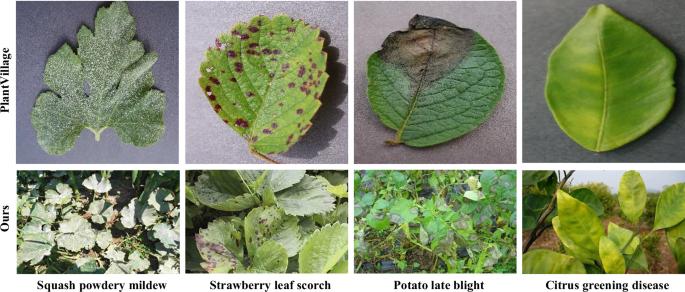

  

  Examples of images of PlantVillage¹⁹ and our PlantSeg dataset. Each image from PlantVillage only contains one leaf and has a uniform background, while images of our dataset feature much more complex backgrounds, various viewpoints, and different lighting conditions.

• Dataset Scale. PlantSeg surpasses existing datasets^21,22 in terms of the number of images, plant types and disease classes. Considering the large variability of plant diseases arising from morphological changes in abnormal growth, appearance, or development, small-scale datasets usually fail to capture the diversity of real-world diseases. In contrast, PlantSeg addresses this issue by introducing 7,774 images across 115 disease categories, thereby better representing the diversity of disease conditions.

Table 1 Summary of existing plant disease image datasets.

In this paper, we showcase the characteristics of PlantSeg and benchmark state-of-the-art segmentation models on plant disease segmentation, demonstrating that our dataset is a comprehensive benchmark for developing plant disease segmentation methods. Benefiting from our newly curated dataset, we are able to train segmentation models that achieve promising generalizable performance on real-world plant disease images. As a result, we effectively tackle the inferior generalization issues of models trained on laboratory datasets or small-scale real-world images. The trained plant disease segmentation models can be applied in automated precision agriculture systems, such as quarantining affected areas within paddocks and adjusting fungicide application rates to minimize the spread of diseases.

Methods

Plant and Disease Category Construction

We first select a number of plants that hold substantial economic and nutritional significance²³. They are high-value profit crops, dietary staple crops, and a diverse range of fruits and vegetables. These plants are representative of the most important plants in agriculture. In total, 34 plant hosts are selected. Then, we identify the critical diseases^24,25,26 associated with each plant host. Notably, as one of the most important crops, wheat is linked to eight distinct diseases, the highest number among the selected plants. Overall, our dataset encompasses images of 69 distinct disease types across 34 plant hosts, resulting in 115 plant diseases. In Fig. 2, we provide an overview of the distribution of the selected plant diseases.

Fig. 2

Hierarchical taxonomy of the PlantSeg dataset, showing the relationships between plants and associated diseases. Colors represent major plant categories, including fruits, vegetables, staple crops, and economically significant plants.

Image acquisition

We collect plant disease images from multiple image search engines. Google Images is used as the primary source due to the broad coverage of global web content. Images from Baidu are included to capture more diverse and region-specific plant disease features, especially from China, which has extensive agricultural regions and diverse crop types. Bing Images further supplements the dataset and enhances diversity across different indexing systems. We use plant disease names as search keywords to retrieve relevant images, which also serve as the category labels in our dataset. Specifically, corresponding Chinese keywords are employed on Baidu for image retrieval. To ensure legal compliance and responsible data usage, we restrict our downloads to images that are explicitly marked as being available under Creative Commons licenses. For each collected image, we record the download URL and license information in the metadata file to ensure transparency and support reproducibility.

Figure 3 illustrates the geolocation distribution of our collected data sources based on IP addresses, demonstrating that our dataset achieves diverse geolocation coverage. All the image data collected here is licensed for free use in research purposes.

Fig. 3

The geolocation distribution of the acquired images. The size of each circle demonstrates the number of images collected from the corresponding locations.

Image cleaning

As images are initially retrieved using disease-specific keywords and organized into folders named after those keywords, we perform data cleaning before the segmentation annotation. Specifically, annotators are instructed to verify whether each image within a folder correctly belongs to the disease category indicated by the folder name. To enhance reliability, each folder is independently reviewed by at least two annotators. The detailed process involves the following steps:

• 1. Annotators independently review each folder, retaining images that correctly match the disease category and discarding those deemed incorrect.

• 2. The results from different annotators are compared to identify disagreements (i.e., one annotator retains an image while the other rejects it).

• 3. Disputed images are submitted to expert plant pathologists for final adjudication.

Segmentation annotation

Afterwards, we establish a segmentation annotation protocol to ensure consistent labeling for diverse disease images. We employ polygons to outline disease-affected areas. Specifically, separate lesions are annotated with individual polygons, and overlapping lesions are treated as a single combined region. For diseases like rust and powdery mildew, their symptoms appear as small, dense clusters on leaves and fruits. Additionally, any deformities in plant leaves or fruits caused by diseases are also annotated. Figure 4 showcases examples annotated by the plant pathologist, and these examples are employed as references for training annotators. Under the guidance of the plant pathologist experts, a team of annotators is trained to perform segmentation annotations.

Fig. 4

Examples of images with annotated polygons on the disease-affected areas.

We used LabelMe (https://github.com/wkentaro/labelme) as our annotation tool. Considering the large domain gap between generic image segmentation and plant disease segmentation, we did not rely on pre-generated masks from automatic tools such as the Segment Anything model²⁷. Instead, we found that annotating from scratch significantly enhances annotation efficiency.

To quantify the inter-annotator agreement, we compute the Foreground-background Intersection over Union (FB-IoU) between the segmentation masks produced by different annotators for the same image. FB-IoU measures the overlap between the annotated foreground regions (i.e., diseased areas) and background regions across annotators. FB-IoU is defined as:

$$FB \mbox{-} IoU=\frac{| \,({M}_{1}=1)\cap ({M}_{2}=1)\,| +| \,({M}_{1}=0)\cap ({M}_{2}=0)\,| }{2\times H\times W},$$

where M₁ and M₂ are binary masks produced by different annotators, and H × W denotes the total number of pixels in the image. If an FB-IoU score of an image is below 0.8, the annotations are considered inconsistent and submitted to domain experts for adjudication. The experts provide feedback to annotators to improve consistency in future annotations. For images with FB-IoU above 0.8, the disagreement is deemed minor, and the final mask is obtained by averaging the different annotations.

Risk management of annotation quality

Before the annotation process, we provide all annotators with standardized training, including written instructions and representative examples. The training phase takes approximately 2 hours. After that, each annotator completes a qualification task involving 50 images sampled from diverse disease categories, which typically requires 4-5 hours. The results are compared against expert annotations using FB-IoU, and only annotators achieving at least 80% consistency are selected. Consequently, 10 annotators are qualified to proceed with the segmentation annotation.

During the annotation process, we conduct risk management in parallel, as illustrated in Fig. 5. Each annotated image is evaluated using FB-IoU-based consistency checks. If an image is flagged as inconsistent, it is submitted to domain experts for adjudication. Approximately 15% of the annotated images undergo this expert review process. Specifically, the time consumption for different diseases significantly varies due to the diverse visual complexities, as shown in Fig. 4. For relatively simple cases such as plum pocket disease, where lesion boundaries are clear and symptoms are visually distinct, annotation typically took around 1 minute per image. In contrast, more complex conditions like cucumber angular leaf spot, which is characterized by subtle color transitions, fragmented lesion boundaries, and background ambiguity, could take upwards of 30 minutes per image. The total time spent on re-annotation is approximately 350 hours.

Fig. 5

Illustration of the curation process of our PlantSeg dataset. It involves three main steps: image acquisition, data cleaning, and annotation. In the image acquisition stage, images were collected from various internet sources using identified keywords and then stored according to their categories. In the data cleaning phase, incorrect images were identified and removed. For the segmentation annotation process, annotators utilized LabelMe to annotate cleaned images. These annotations were subsequently reviewed by experts.

PlantSeg metadata

In this section, we introduce the metadata of PlantSeg, including image names, plant host, disease type, image resolution, annotation file path, mask ratio, URL, license and training/validation/test splits.

Image names

Image names are the unique identifiers for all the images in PlantSeg. In other words, all the metadata of each image in our dataset can be easily retrieved by the image name.

Plants and diseases

PlantSeg includes images of various plant hosts affected by a diverse range of diseases. Specifically, there are 34 distinct host plants and 69 unique disease types. In our dataset, the indices of the plant hosts range from 0 to 33 and the indices of disease types range from 0 to 68. The combinations of these plants and diseases result in 115 unique plant-disease cases. In the mask annotations, we use indices from 0 to 114 to represent the corresponding plant-disease combinations.

URLs

We provide URLs for all images in PlantSeg to promote reproducibility and compliance with copyright regulations. The URLs enable researchers to access the original sources of the images. This also ensures that experiments can be reliably reproduced using the same data.

Licenses

The license information for each collected image is documented in the metadata file to ensure transparency and promote reproducibility.

Annotation files

PlantSeg offers fine-grained segmentation masks for the diseased areas in each image. Each plant disease is assigned a unique class index. The annotation files are stored as grayscale images, where each pixel is assigned to a specific category representing diseases or backgrounds. Moreover, we provide bounding-box annotations by finding a minimal enclosed bounding-box for each connected mask region.

Image-resolutions and mask ratios

The image resolution is provided for better understanding its impacts on disease segmentation and detection. Mask ratios measure the ratio between the labeled pixels and the total number of pixels in an image.

Training/validation/test sets of PlantSeg

We provide a split file that allocates 70% of the image filenames for training, 10% for validation, and 20% for testing. The split file is used to reproduce the segmentation performance results and facilitate fair comparisons among different methods.

Data Records

The PlantSeg dataset is available for download at https://doi.org/10.5281/zenodo.17719108²⁸. The dataset is licensed under the CC BY-NC 4.0. Plant disease images are stored in JPEG format within the images folder, and annotation files are saved in PNG format in the annotations folder. All images and labels are divided into training, validation and test sets with a 70/10/20 split. The meta-information outlined in Table 2 is presented in the Metadata.csv file. An overview of the dataset structure is shown in Fig. 6.

Table 2 Metadata information of our PlantSeg dataset.

Fig. 6

The folder structure of the PlantSeg dataset.

Data Overview

In this section, we provide the statistical analysis on the distributions of disease types, image resolutions, and segmentation mask ratios in PlantSeg.

Plant and disease type distribution

The PlantSeg dataset contains 115 diseases across 34 plant hosts, which are categorized into four major socioeconomic groups: profit crops, staple crops, fruits, and vegetables. We present a detailed circular dendrogram in Fig. 2, showing all plant types in the dataset and their corresponding disease categories. Complementarily, Table 5 summarizes the number of images per disease category, providing a view of the class distribution. As shown in the table, our dataset exhibits imbalance across different plant disease classes. This actually reflects the natural distribution of plant disease occurrence in real-world scenarios, as common diseases are more frequently observed and documented, resulting in more available images. This phenomenon also exists in previous plant disease datasets. Importantly, our dataset includes the most diverse collection of plant disease categories to date, covering a broader range of conditions than existing datasets. While data imbalance is inevitable, our dataset still offers a valuable and realistic benchmark for developing robust methods to address long-tailed distribution and data imbalance challenges in plant disease recognition tasks.

Image resolution distribution

We analyse the distribution of image resolution in PlantSeg and compare it with two widely used plant disease image datasets, i.e., PlantVillage¹⁹ and PlantDoc²⁹, as shown in Fig. 7. To be specific, PlantVillage consists of over 50,000 images, and all the images are captured under controlled laboratory conditions. PlantDoc contains around 2,600 in-the-wild images collected from the internet, but it does not have segmentation masks for the disease-affected regions. The resolution distribution highlights that PlantSeg encompasses a broad range of image resolutions, capturing the variability typically observed in real-world conditions. Although PlantDoc (represented by red points) demonstrates considerable variability, it is on a smaller scale compared to PlantSeg. PlantVillage images are captured under laboratory settings, leading to a consistent resolution across all samples. Figure 7 illustrates that PlantSeg covers a broader range of image resolutions, reflecting the variability of real-world conditions. This highlights the challenges of detecting diseases from field-based images and emphasizes the advantage of our PlantSeg, which has more diverse and variable scales than laboratory-collected data.

Fig. 7

Illustration of the resolution distribution of different datasets. Note that our PlantSeg dataset is superior in terms of resolution diversity and image number. Green, orange and purple markers represent images from PlantSeg, PlantDoc²⁹ and PlantVillage¹⁹, respectively.

Segmentation mask coverage distribution

Figure 8 showcases the distribution of segmentation mask coverage percentages in the PlantSeg dataset. Low coverage indicates that annotated disease areas are relatively small, while high coverage suggests disease-affected areas are large. Overall, the mask coverage in the PlantSeg dataset varies significantly, and the mask ratios of 80% of the images are below 36%.

Fig. 8

Illustration of the distribution of segmentation mask coverage. The horizontal axis represents the percentage of mask coverage with respect to an entire image, and the vertical axis represents the number of images falling in the corresponding percentage. Compared to the existing dataset LDSD²¹, which provides disease segmentation masks, our PlantSeg contains not only a wide range of mask coverage but also significantly more samples.

Technical Validation

Evaluation on PlantSeg

To evaluate the quality of our newly curated plant disease segmentation dataset and establish benchmarks for plant disease segmentation, we performed segmentation methods on the PlantSeg dataset.

Baseline models

We evaluate a wide range of semantic segmentation models to ensure a comprehensive performance assessment on PlantSeg. The selected models represent a diverse set of architectural designs and can be grouped into three categories:

• CNN-based models: MobileNetV3³⁰, PSPNet³¹, Deeplabv3⁴, DeepLabv3+⁵, and CCNet³². MobileNetV3 combines depthwise separable convolutions with neural architecture search and squeeze-and-excitation modules to achieve an optimal trade-off between accuracy and efficiency. PSPNet introduces the Pyramid Pooling Module to aggregate contextual information at multiple spatial scales and capture both local and global features. DeepLabv3 extends this idea through Atrous Spatial Pyramid Pooling (ASPP), which applies dilated convolutions with varying atrous rates in parallel to enlarge the receptive field without sacrificing resolution. DeepLabv3+ incorporates a decoder that fuses low-level and high-level spatial features from ASPP, thereby recovering fine object boundaries. CCNet improves context modeling via criss-cross attention, which efficiently captures global dependencies along horizontal and vertical directions with reduced computational cost.

• Transformer-based models: SegFormer³³, BEiT³⁴, SAN³⁵, and UPerNet³⁶. These models adopt self-attention mechanisms to capture global dependencies, enhancing feature representation and scalability. SegFormer integrates a hierarchical transformer encoder with a simple MLP-based decoder, achieving high accuracy with low latency. BEiT treats image patches as discrete visual tokens and learns to predict masked tokens using a transformer backbone. SAN leverages vision-language models for open-vocabulary segmentation, aligning pretrained features with task-specific outputs via side adapters. UPerNet includes a Feature Pyramid Network (FPN) with a Pyramid Pooling Module (PPM), which leverages multi-level features for hierarchical fusion and global context integration.

• Hybrid models: ConvNeXt³⁷and SegNeXt⁷. The hybrid design leverages the efficiency of CNNs and the contextual modeling strength of transformers to improve segmentation performance. ConvNeXt redesign conventional CNN architectures by incorporating large kernel sizes, inverted bottlenecks, and Layer Normalization from transformers. It achieves competitive performance with transformer-based models while maintaining the simplicity of convolutional operations. SegNeXt integrates attention mechanisms into a purely convolutional framework, combining depthwise separable convolutions and spatial attention for efficient context modeling. It achieves competitive performance with fewer parameters, ideal for real-time and resource-limited scenarios.

All methods were implemented by the PyTorch framework and trained using a Stochastic Gradient Descent (SGD) optimizer with a learning rate of 0.001, momentum of 0.9, and weight decay of 0.0005. Cross-entropy loss was used to optimize the models, and each model was trained with a batch size of 16.

Evaluation metrics

Mean Intersection over Union (mIoU) and Mean Accuracy (mAcc) are employed as our evaluation metrics. mIoU calculates the average Intersection over Union across all classes. Mean Accuracy (mAcc) measures the proportion of correctly classified pixels within each class and then averages these values across all classes. The formulations for these evaluation metrics are as follows:

$${mIoU}_{i}=\frac{1}{C}\mathop{\sum }\limits_{c=1}^{C}\frac{T{P}_{c}}{T{P}_{c}+F{P}_{c}+F{N}_{c}},\qquad mAcc=\frac{1}{C}\mathop{\sum }\limits_{c=1}^{C}\frac{T{P}_{c}}{T{P}_{c}+F{N}_{c}},$$

(1)

where C represents the number of classes. TP_c, FP_c, TN_c, FN_c are the numbers of true positive, false positive, false negative, and true negative pixels for the c-th class, respectively.

Quantitative results

Table 3 presents segmentation results across CNN-based, transformer-based, and hybrid segmentation models on the PlantSeg dataset. Traditional CNNs like MobileNetV3 perform poorly in semantic segmentation due to limited context modeling. PSPNet and DeepLab series improve this by introducing multi-scale context aggregation. CCNet further enhances its capability by capturing directional long-range dependencies. In contrast, transformer-based models consistently outperform CNN-based approaches, primarily due to their ability to model global dependencies and superior feature representation through self-attention. Hybrid architectures explicitly integrate CNN backbones with transformers, enabling efficient local feature extraction while enhancing global context modeling. Notably, ConvNeXt-L obtains the highest overall performance (46.24% mIoU, 59.97% mAcc) with much fewer parameters than many transformer-based models.

Table 3 Quantitative comparisons among different methods on PlantSeg.

Qualitative analysis

Figure 9 illustrates the segmentation predictions produced by representative models across different architectures. CNN-based models often under-segment regions with high shape irregularity, such as elongated or fragmented lesions. This is caused by the limited ability to capture complex global structures of CNNs. In contrast, UPerNet, with its transformer backbone, better captures small and scattered lesions by modeling long-range dependencies. The self-attention mechanism facilitates the extraction of fine-grained and spatially complex features. Furthermore, ConvNeXt demonstrates more coherent and accurate lesion boundaries across diverse lesion types. Its hybrid architecture combines hierarchical convolutional features with enhanced context modeling, further improving its adaptability for disease detection.

Fig. 9

Segmentation predictions produced by representative models from three architectures: CCNet (CNN-based), UperNet (Transformer-based), and ConvNeXt (Hybrid).

However, compared to the human-annotated ground truths, some areas with minor symptoms are often overlooked by the baseline methods. For instance, in the bottom row of Fig. 9, although ConvNeXt successfully captures wilted leaves, it fails to correctly segment the collapsed stems. Moreover, benign areas tend to be included in their predicted masks when disease symptoms are exhibited nearby, as seen in the second row. This suggests that ConvNext tends to predict masks to cover larger areas than the ground-truth regions.

Condition-specific performance evaluation

We assess model robustness by analysing performance across three key lesion characteristics: size, shape irregularity, and proximity to leaf boundaries.

Impact of lesion sizes

To better understand how lesion sizes influence segmentation performance, we construct a scatter plot (Fig. 10). It illustrates the relationship between the ground truth mask ratio and the IoU predicted by ConvNeXt. The scatter plot reveals that when a lesion area occupies only a small portion of the image, the model often produces inaccurate predictions. As the mask ratio increases, its segmentation results become better. Overall, lesion size has a noticeable impact on segmentation performance. Larger lesions are generally easier for the model to detect, while small lesions present a significant challenge for accurate segmentation, often leading to inferior performance.

Fig. 10

Left: IoU shows a generally positive correlation with the ground truth mask ratio. Right: Examples with small lesions, where the model struggles in detecting diseased regions.

Impact of shape irregularity

To investigate the relationship between lesion shape irregularity and segmentation performance, we introduce a convexity-based metric to quantify shape irregularity. Specifically, the convex hull is the minimal convex polygon that entirely contains the lesion region. Given a binary lesion mask ${\mathcal L}$, we denote its area as $A( {\mathcal L} )$, and the area of its convex hull as $A(CH( {\mathcal L} ))$. The convex hull ratio is defined as:

$$CHR=\frac{A( {\mathcal L} )}{A(CH( {\mathcal L} ))},$$

(2)

When the shape exhibits high irregularity and fragmentation, the convex hull ratio tends to be low. In contrast, more regular and compact shapes yield higher convex hull ratios, approaching 1. As shown in Fig. 11, lower convex hull ratios are consistently associated with reduced segmentation performance. In addition, the presented examples demonstrate that regular-shaped lesions with high convex ratios are segmented more accurately, whereas highly irregular lesions yield poor results. These results indicate that higher shape irregularity harms segmentation accuracy.

Fig. 11

Left: IoU positively correlates with the convex hull ratio. Right: Examples in which regular-shaped lesions are well segmented, whereas irregular and fragmented lesions exhibit poor segmentation performance.

Impact of lesion locations

Since leaf boundaries are not annotated in our dataset, the spatial relationship between lesions and leaf boundaries is difficult to quantify. Instead, we conduct a qualitative analysis of segmentation results by randomly selecting 100 images. It is observed that lesions located near the center of a leaf are much easier to segment compared to those positioned near the leaf edges. The presented examples, as shown in Fig. 12, indicate that lesions located within leaves yield more accurate segmentation results, while those close to the leaf edges are more likely to be under-segmented or completely missed. This discrepancy may be attributed to the fact that lesions near the leaf edges are more likely to be confused with the background. In contrast, lesions in the central regions typically exhibit simpler backgrounds that facilitate segmentation.

Fig. 12

Lesions near the center of the leaf are segmented more accurately, while those near the edges tend to be under-segmented or missed.

Failure case analysis

We examine the prediction of different samples and identify several representative types of failure, as shown in Fig. 13. As shown in case 1, the ground truth annotations indicate a large number of small disease lesions, which are marked as red dots. However, the model (i.e., ConvNeXt) fails to detect many of them. This is likely due to the extremely small size of the lesions, which occupy only about 1% of the image. In addition, the complex background makes it challenging for the model to distinguish lesion areas from the surroundings. Case 2 shows the model accurately localizes diseased regions but misclassifies them due to high visual similarities. For example, peach scab is mistaken for apple scab because both exhibit clustered dark spots on fruit surfaces. Similarly, corn northern leaf spot is misclassified as corn gray leaf spot, as both show elongated lesions along leaf veins. Although spatial predictions are correct, this misclassification leads to an IoU of 0, demonstrating the challenge of distinguishing diseases with similar visual characteristics. In case 3, although the model correctly classifies apple mosaic virus and apple scab, the predicted regions only partially match the ground truth. This is because strong illumination reduces contrast, leading the model to overestimate the affected region.

Fig. 13

Illustrations of representative failure cases: missed detection, misclassification and mislocalization.

These results imply that state-of-the-art segmentation models might still struggle with complex disease symptoms under different scenarios. Our dataset offers a valuable and realistic benchmark for practical plant disease method development.

Discussion on model limitations and potential improvements

The failure cases expose inherent weaknesses in current models, motivating several directions for improvement. For small and sparse lesions, the key challenge lies in their limited visual saliency, which often leads to under-segmentation. This issue can be alleviated by designing loss functions that place greater emphasis on small objects to counter the bias toward dominant background regions. Moreover, targeted data augmentation strategies can increase the occurrence of small and sparse lesions, improving the model’s robustness to such difficult cases.

For irregular and fragmented lesions, the primary difficulty is preserving structural continuity within connected regions. Conventional pixel-wise predictions often ignore local affinity, resulting in broken or incomplete masks for elongated or perforated lesion shapes. Following the insight from the affinity-based approach iShape³⁸ designed for irregular object segmentation, the importance of modeling pixel connectivity and spatial coherence is emphasized. Learning such relational structures allows the model to better capture discontinuous lesion patterns.

Lesions located near leaf edges are often misclassified due to confusion with the background. In addition, specular highlights or visually similar disease patterns can also lead to misidentification. These errors mainly arise from insufficient inter-class discrepancy, where the feature representations of different categories are not well separated. Strengthening the model’s fine-grained representation capacity through contrastive or class-aware learning objectives can enhance the separability between visually similar categories. Additionally, integrating multimodal information such as textual descriptions can provide complementary discriminative cues, helping the model better distinguish lesions of different disease types from background noise or visually similar categories.

Evaluating joint supervision of masks and boxes

All the segmentation masks in our dataset are manually annotated, and the bounding boxes are generated as the minimal enclosed rectangles of these masks. In order to further investigate the benefits of the derived bounding boxes, we conduct additional experiments using Mask R-CNN under two settings: (1) training with segmentation masks only, and (2) training with both masks and bounding boxes. As shown in Table 4, we observe that Mask R-CNN trained with both masks and bounding boxes yields better performance. This result suggests that bounding boxes provide beneficial supervision during training. Compared to using only pixel-wise masks, the additional spatial constraints introduced by bounding boxes enhance the quality of region proposals and improve localization. In addition, bounding boxes offer explicit instance-level cues, thus facilitating the separation of adjacent or overlapping lesions, especially in complex and crowded scenes.

Table 4 Performance of Mask R-CNN trained with and without bounding boxes.

Table 5 The image number of each plant disease class in the PlantSeg dataset.

References

Shoaib, M. et al. An advanced deep learning models-based plant disease detection: A review of recent research. Frontiers in Plant Science 14, 1158933 (2023).
Agrios, G. N. Plant pathology (2005).
Shafi, U. et al. Precision agriculture techniques and practices: From considerations to applications. Sensors 19, 3796 (2019).
Chen, L.-C., Papandreou, G., Schroff, F. & Adam, H. Rethinking atrous convolution for semantic image segmentation. arXiv preprint arXiv:1706.05587 (2017).
Chen, L.-C., Zhu, Y., Papandreou, G., Schroff, F. & Adam, H. Encoder-decoder with atrous separable convolution for semantic image segmentation. In Proceedings of the European conference on computer vision (ECCV), 801–818 (2018).
Kirillov, A., Wu, Y., He, K. & Girshick, R. Pointrend: Image segmentation as rendering. In Proceedings of the IEEE/CVF conference on computer vision and pattern recognition, 9799–9808 (2020).
Guo, M.-H. et al. Segnext: Rethinking convolutional attention design for semantic segmentation. Advances in Neural Information Processing Systems 35, 1140–1156 (2022).
Zhou, B. et al. Semantic understanding of scenes through the ade20k dataset. International Journal of Computer Vision 127, 302–321 (2019).
Cordts, M. et al. The cityscapes dataset for semantic urban scene understanding. In Proceedings of the IEEE conference on computer vision and pattern recognition, 3213–3223 (2016).
Lin, T.-Y. et al. Microsoft coco: Common objects in context. In Computer Vision–ECCV 2014: 13th European Conference, Zurich, Switzerland, September 6-12, 2014, Proceedings, Part V 13, 740–755 (Springer, 2014).
Bhatti, M. A. et al. Advanced plant disease segmentation in precision agriculture using optimal dimensionality reduction with fuzzy c-means clustering and deep learning. IEEE Journal of Selected Topics in Applied Earth Observations and Remote Sensing (2024).
Jafar, A., Bibi, N., Naqvi, R. A., Sadeghi-Niaraki, A. & Jeong, D. Revolutionizing agriculture with artificial intelligence: plant disease detection methods, applications, and their limitations. Frontiers in Plant Science 15, 1356260 (2024).
Wang, D., Wang, J., Li, W. & Guan, P. T-cnn: Trilinear convolutional neural networks model for visual detection of plant diseases. Computers and Electronics in Agriculture 190, 106468 (2021).
Li, J. et al. An improved yolov5-based vegetable disease detection method. Computers and Electronics in Agriculture 202, 107345 (2022).
Xie, X. et al. A deep-learning-based real-time detector for grape leaf diseases using improved convolutional neural networks. Frontiers in plant science 11, 751 (2020).
Savarimuthu, N. et al. Investigation on object detection models for plant disease detection framework. In 2021 IEEE 6th international conference on computing, communication and automation (ICCCA), 214–218 (IEEE, 2021).
Wei, T., Chen, Z. & Yu, X. Snap and diagnose: An advanced multimodal retrieval system for identifying plant diseases in the wild. In Proceedings of the 6th ACM International Conference on Multimedia in Asia, 1-3 (2024).
Shoaib, M. et al. Deep learning-based segmentation and classification of leaf images for detection of tomato plant disease. Frontiers in Plant Science 13, 1031748 (2022).
Hughes, D., Salathé, M. et al. An open access repository of images on plant health to enable the development of mobile disease diagnostics. arXiv preprint arXiv:1511.08060 (2015).
Zhang, Y., Song, C. & Zhang, D. Deep learning-based object detection improvement for tomato disease. IEEE access 8, 56607–56614 (2020).
Şener, A. & Ergen, B. Advanced cnn approach for segmentation of diseased areas in plant images. Journal of Crop Health 76, 1569–1583 (2024).
Prashanth, K., Harsha, J. S., Kumar, S. A. & Srilekha, J. Towards accurate disease segmentation in plant images: A comprehensive dataset creation and network evaluation. In Proceedings of the IEEE/CVF Winter Conference on Applications of Computer Vision, 7086–7094 (2024).
Dulloo, M., Hunter, D. & Leaman, D. Plant diversity in addressing food, nutrition and medicinal needs. Novel plant bioresources: applications in food, medicine and cosmetics 1–21 (2014).
Strange, R. N. & Scott, P. R. Plant disease: a threat to global food security. Annu. Rev. Phytopathol. 43, 83–116 (2005).
Sawicka, B., Egbuna, C., Nayak, A. K. & Kala, S. Chapter 2 - plant diseases, pathogens and diagnosis. In Egbuna, C. & Sawicka, B. (eds.) Natural Remedies for Pest, Disease and Weed Control, 17–28, https://doi.org/10.1016/B978-0-12-819304-4.00002-6 (Academic Press, 2020).
Figueroa, M., Hammond-Kosack, K. E. & Solomon, P. S. A review of wheat diseases–a field perspective. Molecular plant pathology 19, 1523–1536 (2018).
Kirillov, A. et al. Segment anything. In Proceedings of the IEEE/CVF International Conference on Computer Vision, 4015–4026 (2023).
Wei, T. A large-scale in-the-wild dataset for plant disease segmentation, https://doi.org/10.5281/zenodo.17719108 (2024).
Singh, D. et al. Plantdoc: A dataset for visual plant disease detection. In Proceedings of the 7th ACM IKDD CoDS and 25th COMAD, 249–253 (2020).
Howard, A. et al. Searching for mobilenetv3. In Proceedings of the IEEE/CVF international conference on computer vision, 1314–1324 (2019).
Zhao, H., Shi, J., Qi, X., Wang, X. & Jia, J. Pyramid scene parsing network. In Proceedings of the IEEE conference on computer vision and pattern recognition, 2881–2890 (2017).
Huang, Z. et al. Ccnet: Criss-cross attention for semantic segmentation. In Proceedings of the IEEE/CVF international conference on computer vision, 603–612 (2019).
Xie, E. et al. Segformer: Simple and efficient design for semantic segmentation with transformers. Advances in neural information processing systems 34, 12077–12090 (2021).
Bao, H., Dong, L., Piao, S. & Wei, F. Beit: Bert pre-training of image transformers. In International Conference on Learning Representations (2022).
Xu, M., Zhang, Z., Wei, F., Hu, H. & Bai, X. Side adapter network for open-vocabulary semantic segmentation. In Proceedings of the IEEE/CVF Conference on Computer Vision and Pattern Recognition, 2945–2954 (2023).
Xiao, T., Liu, Y., Zhou, B., Jiang, Y. & Sun, J. Unified perceptual parsing for scene understanding. In Proceedings of the European conference on computer vision (ECCV), 418–434 (2018).
Liu, Z. et al. A convnet for the 2020s. In Proceedings of the IEEE/CVF conference on computer vision and pattern recognition, 11976–11986 (2022).
Yang, L. et al. iShape: A first step towards irregular shape instance segmentation. arXiv preprint arXiv:2109.15068 (2021).
Moupojou, E. et al. Fieldplant: A dataset of field plant images for plant disease detection and classification with deep learning. IEEE Access 11, 35398–35410 (2023).
Wei, T., Chen, Z., Huang, Z. & Yu, X. Benchmarking in-the-wild multimodal plant disease recognition and a versatile baseline. In Proceedings of the 29th ACM international conference on multimedia (2024).
He, K., Zhang, X., Ren, S. & Sun, J. Deep residual learning for image recognition. In CVPR (2016).
Dosovitskiy, A. et al. An image is worth 16 × 16 words: Transformers for image recognition at scale. In International Conference on Learning Representations (2021).
Liu, Z. et al. Swin transformer: Hierarchical vision transformer using shifted windows. In Proceedings of the IEEE/CVF international conference on computer vision, 10012–10022 (2021).
He, K., Gkioxari, G., Dollár, P. & Girshick, R. Mask r-cnn. In Proceedings of the IEEE international conference on computer vision, 2961–2969 (2017).
Acknowledgements
We thank all the people involved in image acquisition, annotation and reviewing. We also thank the people who contributed to this paper. This work was supported by Australian Research Council CE200100025, DP230101196, and Grains Research and Development Corporation UOQ2301-010OPX.
Author information
Authors and Affiliations
Contributions
Tianqi Wei designed the study, built the dataset, conducted experiments and wrote the manuscript. Zhi Chen designed the study, built the dataset and wrote the manuscript. Xin Yu designed the study and revised the manuscript. Scott Chapman and Paul Melloy supervised the annotation process, validated the data and reviewed the manuscript. Zi Huang administrated the project, offered resources and reviewed the manuscript.
Corresponding author
Ethics declarations
Competing interests
The authors declare no competing interests.
Additional information
Publisher’s note Springer Nature remains neutral with regard to jurisdictional claims in published maps and institutional affiliations.
Rights and permissions
Open Access This article is licensed under a Creative Commons Attribution-NonCommercial-NoDerivatives 4.0 International License, which permits any non-commercial use, sharing, distribution and reproduction in any medium or format, as long as you give appropriate credit to the original author(s) and the source, provide a link to the Creative Commons licence, and indicate if you modified the licensed material. You do not have permission under this licence to share adapted material derived from this article or parts of it. The images or other third party material in this article are included in the article’s Creative Commons licence, unless indicated otherwise in a credit line to the material. If material is not included in the article’s Creative Commons licence and your intended use is not permitted by statutory regulation or exceeds the permitted use, you will need to obtain permission directly from the copyright holder. To view a copy of this licence, visit http://creativecommons.org/licenses/by-nc-nd/4.0/.
About this article
Cite this article
Wei, T., Chen, Z., Yu, X. et al. A Large-Scale In-the-wild Dataset for Plant Disease Segmentation. Sci Data 13, 205 (2026). https://doi.org/10.1038/s41597-025-06513-4
Received:
Accepted:
Published:
Version of record:
DOI: https://doi.org/10.1038/s41597-025-06513-4