An efficient intelligent transportation system for traffic flow prediction using meta-temporal hyperbolic quantum graph neural networks

Abstract

Intelligent Transportation Systems (ITS) necessitate scalable, real-time, and adaptive traffic flow prediction models to enhance urban mobility and alleviate congestion. Conventional Graph Neural Network methodologies encounter difficulties in managing extensive road networks, long-range temporal relationships, and computing efficiency for real-time applications. An innovative deep learning framework named Meta Temporal Hyperbolic Quantum Graph Neural Networks that integrates hyperbolic embeddings, meta learning, quantum graph, Neural Ordinary Differential Equation (NODEs) to improve the ITS Performance. Across many cities, meta learning facilitates swift adaptation with minimum retraining whereas hyperbolic graph embeddings efficiently depict hierarchical route configurations The usage of Quantum Graph Neural Networks (QGNNs) enhances graph-based scheming, enabling real-time traffic flow to forecast for extensive networks. Also, NODEs summarize ongoing traffic progress, enhancing precision under dynamic sceneries. Datasets like Los-loop and SZ-taxi datasets are validated by experiments which highlights the impact of the proposed MTH-QGNN model, acquiringamean value RMSE of 4.5 and MAE of 3.5, ensuring minimal prediction error. MTH-QGNN model constantly sustained accuracy above 80% and R² values exceeding 83%, representing robust predictive trustworthiness. MTH-QGNN effectively captures complex spatiotemporal traffic patterns with a variance score above threshold value.

Introduction

Considering, growing quantity of automobiles on the road, modern transportation schemes face significant challenges such as gridlock, frequent accidents, thenconservational deterioration. When taking action for above issue rise induced demand which worsening traffic conditions rather than improving them^1,2. To enhance mobility and optimize road network efficiency, more intelligent data driven systems needed.

Advanced analytics, enhanced communication technology, and Intelligent Transportation Systems (ITS)³ have become revolutionary solutions. ITS integrates 5G communication, IoT-based sensors, and AI-driven decision-making to enhance traffic flow, minimize congestion, and improve road safety. This advanced framework not only enhances travel efficiency but also contributes to reducing accident risks, lowering carbon emissions, and improving passenger satisfaction^4,5. To provide better traffic management and help policymakers, transportation authority, aspects of ITS helps to predict traffic flow prediction^6,7. Road Traffic accidents remain a global challenge, which highlighting the necessity for consistent predicting techniques to safeguard road users and offer more cost-effective travel^8,9,10.

Traditionally, traffic prediction relied on parametric models such as time-series analysis, Kalman filtering¹¹, and Auto-Regressive Integrated Moving Average (ARIMA)¹¹, which analyze historical data to forecast future conditions. But since traffic flow is unpredictable and nonlinear¹², nonparametric models^13,14,15,16 like Random Forest (RF), Bayesian Algorithms (BA), K-Nearest Neighbor (KNN), Principal Component Analysis (PCA), and Support Vector Machines (SVMs) have been introduced to improve prediction accuracy.

By the rise of big data and Deep Learning (DL) models, more advanced neural network architectures have revolutionized traffic prediction. Early approaches such as Back-Propagation Neural Networks (BPNN)¹⁷ paved the way for modern DL models, including Convolutional Neural Networks (CNNs), Recurrent Neural Networks (RNNs), Graph Convolutional Network (GNN), Long Short-Term Memory (LSTM), Restricted Boltzmann Machines (RBM), Deep Belief Networks (DBN), and Stacked Auto-Encoders (SAE)^18,19,20,21. For better congestion control, route optimization, above specified model enables ITS and also develop large quantity of dynamic statistics efficiently. Even traditional traffic prediction models are struggled to handle complex dynamic and large-scale urban road networks. With the beginning of deep learning, mainly Graph Neural Networks (GNNs)^22,23, ITS has seen considerable advancements in traffic flow prediction. However, existing GNN-based models face scalability, real-time adaptation, and long-term forecasting limitations, necessitating more advanced methodologies.

To address these challenges, Meta-Temporal Hyperbolic Quantum Graph Neural Networks (Meta-Temporal H-QGNNs) is proposed, an innovative framework that integrates meta-learning, hyperbolic graph embeddings, quantum graph computation, and neural ordinary differential equations (Neural ODEs) to enhance traffic flow prediction and management. Meta-learning approaches, such as the Bayesian Meta-Learning framework, have demonstrated adaptability in capturing spatial–temporal variations in traffic data, enabling models to generalize across different regions with minimal retraining.

Bayesian Meta Learning framework experiments the adaptability of spatial–temporal variations in traffic data to allowing models to simplify across various regions with minimal retraining. Also, frameworks like STDA used to improve minimal traffic prediction which handle scenarios with limited data. Graph neural networks (GNNs) application such as hyperbolic embedding has improved the notation of hierarchical road structures, easing more accurate long-term traffic forecasting. The constraints of traditional traffic prediction models include the inability to incorporate intricate spatial–temporal connections. Inadequate generalization across various locales. Elevated computational expenses for real-time applications. Insufficient resilience to data sparsity. Scalability challenges in extensive networks.

Moreover, the combination of quantum computing values into GNNs, as seen in the Temporal-Spatial Quantum Graph Convolutional Neural Network, has enhanced calculations, making real-time predictions in large-scale networks feasible. Furthermore, the use of Neural ODEs permits for continuous-time modeling of traffic dynamics, taking the fluid development of traffic flow more exactly than traditional discrete models. This continuous approach brings into line with the characteristic nature of traffic systems, leading to better-quality prediction accuracy and responsiveness. Collectively, these advancements have culminated in the development of sophisticated models that are not only scalable and adaptive but also capable of providing real-time, uncertainty-aware traffic management solutions.

The key highlights of proposed work are:

• 1. A GNN system based on meta-learning that requires less retraining to adjust traffic models across several cities.

• 2. Road network representation progressed by hyperbolic graph embeddings and long-term traffic forecasting.

• 3. For large-scale ITS applications significantly reducing the processing time by quantum-enhanced GNN computation.

• 4. Neural ODE-based continuous traffic flow model helps to improve prediction accuracy for real-time traffic variations.

• 5. Extensive experiments on traffic datasets, showing notable analytical performance in prediction, data flexibility, and computational efficiency compared to existing ITS models.

Furtherly, Section “Related work” explains a completeevaluation of existing traffic flow prediction methods in ITS, including traditional statistical approaches, machine learning models, and deep learning techniques. Section “Proposed methodology” then summaries the architecture of the proposed ITS-based traffic prediction framework, detailing its components, data sources, and processing techniques. Section “Quantum Graph Neural Network (QGNN)” focuses on the implementation, describing the hardware and software infrastructure used, while also evaluating the effectiveness of different ML/DL models based on prediction accuracy and real-time processing routine. To conclude, Section “Neural Ordinary Differential Equation (NODE) Layer” précises the important findings then emphasizes the transformative potential of ITS-based predictive models in optimizing urban traffic management.

Related work

Conventional and advanced approaches are discussed detail along with analysis of existing traffic prediction methods in the following section. Determine the role of Intelligent Transport Systems (ITS) in traffic prediction helps to focus on integrate the dynamic data from sensors. In addition to this, key challenges such as processing speed, reliability of data, heterogeneity of data are also discussed. New edge computing method based on deep learning introduced by Wang et al.²⁴, are considered. Due to traffic hike traditional cloud based ITS Solutions face challenge in storage, communication, surveillance demands. To resolve above stated issue, the proposed methods use edge computing where model YOLOv3 applied for vehicle detection and DeepSORT used for identifying multi-object. Edge device like Jetson TX2 organized for implementation. This method gives the dynamic traffic flow detection with huge accuracy rate while reduce the reliance on cloud computing.

Yan et al.²⁵ highlight the position of traffic flow prediction in Intelligent Transportation Systems (ITS). Traditional graph-based models struggle to capture hidden spatial and temporal dependencies. To solve this, GECRAN (Graph Embedding Convolutional Recurrent Attention Network) was proposed, which consists of three key components: PGEM (captures spatial correlations), GCRN (handles temporal dependencies), and ATTM (identifies long-term patterns). Experiments on four real-world datasets show that GECRAN improves prediction accuracy by 2.35%, 3.55%, and 4.22% across three-time steps.

Vo et al.²⁶ proposed a new hybrid approach calledFastVariational Mode Decomposition(FVMD) Whale Optimization Algorithm (WOA) combined with optimization methods such as the genetic algorithm (GA) to improve traffic flow prediction in 5G-enabled Intelligent Transportation Systems (ITS). This amalgamation agrees the model to distinctly handle each decomposed traffic sub-sequence. Additionally, advanced deep learning models—such as LSTM, BiLSTM, GRU, and BiGRU—are used to capture complex temporal dependencies in traffic data. RMSEs model achieves 152.43 and 7.91, corresponding to accuracy improvements of 3.44% and 12.87% over existing methods, while also reducing processing time and enhancing system adaptability.

Federated learning-based system for short-term traffic flow prediction (TFP) in Intelligent Transportation Systems (ITS) proposed by Al-Huthaifi et al.²⁷. With the help of spatial–temporal graph attention networks (AGAT) overcomes challenges in centralized systems, such as slow training, high costs, and privacy risks. The method includes community-based subnetwork division, local training, parameter updates, and global aggregation. Experiments conducted over two real-world datasets shows that FedAGAT attains high accuracy, closely same as real traffic patterns while reducing training time.

Ou et al.²⁸ presented a methodology for forecasting interpretable traffic flow that blends interpretable machine learning with ensemble learning. It uses tree-ensemble algorithms for accurate forecasting and applies six interpretability techniques to analyze models from the neighbourhood and broad view. The framework ensures reliability with real-world traffic patterns and performs well against statistical, shallow learning, and deep learning models. For Intelligent Transportation Systems (ITS) applications it allows customization with different algorithms, making it a reliable solution.

Harrou et al.²⁹ established a wavelet-based denoising approach combined with Recurrent Neural Networks (RNNs) to improve traffic flow prediction in Intelligent Transportation Systems (ITS). The method influences Long Short-Term Memory (LSTM) and Gated Recurrent Unit (GRU) models to control nonlinear and time-based dependencies. Exponential smoothing and wavelet filtering (Symlet and Haar) help eliminate noise from traffic data. By achieving average scores of 0.982 and 0.9811, the approach significantly improves prediction accuracy tested on California highway datasets (I-880 and I-80),

Zhao et al.³⁰ proposed the Spatio-temporal Causal Graph Attention Network (STCGAT) to improve traffic flow prediction by overcoming the limitations of traditional Graph Neural Network (GNN) and Recurrent Neural Network (RNN)-based methods. STCGAT dynamically creates subgraphs of spatial adjacency for every time step. using a node embedding technique, eliminating the need for prior geographic data and simplifying graph modeling. It also features a causal temporal correlation module, which integrates node-adaptive learning, graph convolution, and local/global causal temporal convolution modules to capture complex spatiotemporal dependencies. Final results expressed that STCGAT outdoes baseline models on traffic datasets.

Long Short-Term Memory (LSTM)-based prediction model for Intelligent Transportation Systems (ITS) presented by Lu et al.³¹. The approach incorporates with Variational Mode Decomposition (VMD) to handle non-stationary and highly random time series signals. The model is a reliable option for short-term traffic flow prediction since results comparisons prove that it endlessly hits standard methods diagonally a variety of performance parameters.

Chen et al.³² discussed about model termed Graph Attention Network with Spatial–Temporal Clustering (GAT-STC) to recover traffic flow forecasting in Intelligent Transportation Systems (ITS). GAT-STC integrates both recent and periodic aware features for more reliable predictions. In order to improve learning efficiency, a spatial–temporal clustering algorithm groups nodes according to traffic statuses and trends, while a distance-based Graph Attention Network (GAT) detects hidden spatial patterns among neighbouring nodes. In terms of accuracy and efficiency, three public traffic datasets, tested and hits five baseline models.

To improve prediction accuracy in Intelligent Transportation Systems (ITS), Zhang et al.³³ proposed a traffic flow forecasting method using Quantum Particle Swarm Optimization (QPSO). The model assimilates a genetic simulated annealing algorithm within QPSO to augment initial cluster centres and fine-tune the limitations of a Radial Basis Neural Network (RBFNN). RBFNN’s function approximation capability, the model produces exact traffic flow predictions.

Chen et al.³⁴ proposed new method for predicting traffic flow using Dynamic Spatial Temporal Trend Transformer to determine spatio temporal correlations in dynamic network traffic.Huang et al.³⁵ introduced new Intelligent Transportation Systems (ITS) using Multi Personality Multi Agent Meta Reinforcement Learning (MPMA-MRL) framework. The proposed application was implemented and evaluated in EV charging and parking stations. By utilizing this framework it reduces the waiting time in both the stations.

Liu and Shin³⁶ provided an extensive analysis of TFP (Traffic Flow Prediction) techniques within the framework of ITS (Intelligent Transportation Systems). Their research classifies the forecasting methodologies into conventional statistical models, ML (Machine Learning), and novel DL methods. While doing so, they offer a comprehensive overview of the advancement of traffic modeling systems.

Li and Wang³⁷ introduced a DL-based algorithm for real-time TFP, specifically designed for intelligent highway systems. The model utilizes time-series traffic data to improve the precision and responsiveness of predictions in changing traffic situations.

Dou and Chen³⁸ investigated the enhancement of DL methodologies for traffic flow forecasting in Intelligent Transportation Systems by refining model architectures. They investigated how improvements like attention processes and residual learning could enhance model performance and generalization.

Yan³⁹ performed an investigation on the forecasting and improvement of urban traffic flow with DL techniques. This study combines predictive modeling with real-time optimization techniques to enhance urban mobility via intelligent traffic management. Comparative simulations including QPSO-RBF, shows that the approach decreases prediction errors while safeguarding stable and reliable prediction, making it a valued ITS solution (See Table 1).

Table 1 Research gap among traffic flow forecasting using ML and DL methods in ITS.

Traffic flow prediction in ITS has been improved by a number of innovative techniques. By optimizing DL models like YOLOv3 and DeepSORT, edge computing diminishes dependence on the cloud and enables real-time monitoring. Whereas hybrid approaches (FVMD-WOA-GA) join optimization techniques to enhance accuracy, graph-based models (GECRAN, STCGAT) capture spatiotemporal relationships. Decentralized, privacy-preserving predictions are guaranteed by federated learning (FedAGAT), while interpretability-driven models employ tree ensembles to develop deeper perceptions. Methods like QPSO with RBFNN and wavelet-based denoising with RNNs which are efficiently handled dynamic traffic patterns.

Multifaceted spatiotemporal dependencies, high computation costs, and real-time processing limits are still obstacles in spite of recent progressions. In order to progress forecast accuracy while dropping overhead, MTH-QGNNs associate hyperbolic geometry, quantum computing, and meta-learning. A scalable, real-time solution for ITS applications is guaranteed by meta-learning enabling adaptation, quantum graph learning speeding up training, and hyperbolic embeddings capturing complicated traffic dynamics.

Proposed methodology

This section introduces the proposed MTH-QGNN(Meta-Temporal Hyperbolic Quantum Graph Neural Network) framework for traffic prediction in ITS. The MTH-QGNN model is developed to address its complex spatiotemporal dynamics of traffic flow through the integration of various advanced learning components, as illustrated in Fig. 1.

Fig. 1

overall schematic of proposed MTH-QGNNs in ITS.

Sequential Procedure Overview of the MTH-QGNN Framework and is shown in Fig. 2:

Fig. 2

Flow diagram of proposed MTH-QGNNs in ITS.

• 1. Data Acquisition: Traffic data is obtained from two actual sources:

  • GPS trajectories (derived from the SZ-Taxi dataset)

  • Loop detectors (sourced from the Los-Loop dataset)

• 2. Data Preparation: The unprocessed traffic data is converted into organized input:

  • Road network graphs are generated by map-matching techniques or established sensor locations.

  • Feature extraction identifies essential characteristics including vehicle speed, traffic volume, and historical patterns.

• 3. Hyperbolic Embedding Layer

  • The Euclidean Road network graph is mapped into hyperbolic space.

  • This approach more effectively maintains hierarchical linkages among roads (e.g., highways versus small streets).

• 4. Quantum Graph Neural Network (QGNN)

  Spatial links are represented by quantum-inspired graph convolutions, facilitating sophisticated message transmission between nodes (roads) in the graph.

• 5. Neural Ordinary Differential Equation (NODE) Layer

  The temporal progression of traffic is represented as a continuous process utilizing NODEs. This enhances the accuracy of predicting future traffic situations over extended durations.

• 6. Meta-Learning Module

  A meta-learner optimizes the foundational MTH-QGNN model, enabling rapid adaptation to novel traffic patterns with little retraining, hence enhancing the system’s efficiency for deployment across several cities.

• 7. Prediction of Traffic Flow

  The ultimate result is a forecast of traffic flow that facilitates real-time traffic regulation, congestion mitigation, and route optimization within ITS contexts and the process is shown in Fig. 3.

  Fig. 3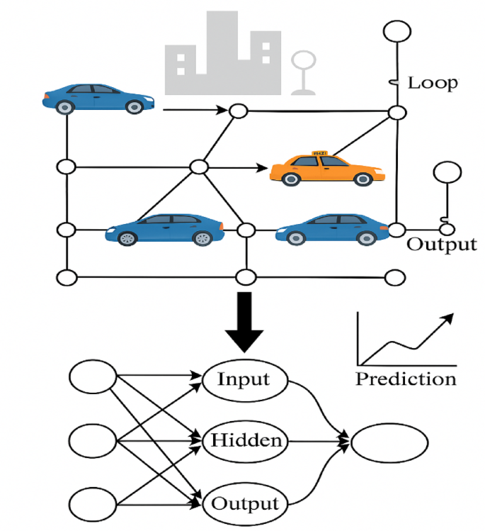

  

  Conceptual Diagram of Traffic Flow and NN-Based Prediction.

Fundamental concepts

In the following subsection, fundamental concepts of road network and formally defines the traffic flow calculation problem has been defined in detail.

Road network structure

A road network consists of interconnected road segments monitored by road sensors, which are deployed at specific locations to gather real-time traffic statistics such as vehicle speed, traffic volume, and congestion levels. These sensors play a vitalcharacter in Intelligent Transportation Systems (ITS) by continuously capturing and transmitting traffic flow information for analysis.

To formally represent a road network, it is modelled as a directed graph shown in Eq. (1)

$$Gh=(Ve,Ed,Am)$$

(1)

where $Ve=\{{ve}_{1},{ve}_{2},\dots ,{ve}_{N}\}$ is the set of road sensors, with $N=|Ve|$ denoting the total number of sensors. $Ed\subseteq Ve\times Ve$ represents the set of edges that define the connectivity between road sensors. Individually edge ${ed}_{ij}\in Ed$ represents a focusedconnection between two road sensors ${ve}_{i}$ and ${ve}_{j}$, indicating traffic flow between those segments.$Am\in {\mathbb{R}}^{N\times N}$ is the adjacency matrix, where each element ${Am}_{ij}$ indicates whether there is a direct road connection between sensor ${ve}_{i}$ and ${ve}_{j}$. If a connection exists, ${Am}_{ij}=1$, otherwise ${Am}_{ij}=0$.

Various road segments spatial interaction is precisely measured by graph-based model. To analyze the geographical and time traffic patterns, a sensor network grouped with interconnected nodes which form graph topology. To predict the future condition, significant data patterns should identify in sensor by apply the graph-based learning algorithms.

Problem Definition

Analyzing past traffic data to project future traffic conditions is known as traffic prediction.Capturing the Traffic flow’s periodic evolution and the three-dimensional connections between road segments is the primary challenge.

Definition 1

Road Signal Representation

At any given time, interval $t$, the traffic state at sensor ${ve}_{i}$ is represented as Eq. (2):

$${a}_{i}^{t}\in {\mathbb{R}}^{F}$$

(2)

where F denotes the number of features recorded by the sensor, such as traffic speed, vehicle count, and road occupancy. The overall road network’s state at time t is defined as Eq. (3):

$${A}^{t}=[{a}_{1}^{t},{a}_{2}^{t},\dots ,{a}_{N}^{t}]\in {\mathbb{R}}^{N\times F}$$

(3)

which encapsulates the traffic conditions at all N sensors.

Definition 2

Traffic Flow Prediction

Predicting future traffic conditions using historical traffic observations is the aim of traffic forecasting. Given the traffic states recorded over the last ${Tc}_{p}$ time intervals in Eq. (4):

$$A=[{A}^{t-{Tc}_{p}+1},{A}^{t-{Tc}_{p}+2},..,{A}^{t}]\in {\mathbb{R}}^{{Tc}_{p}\times N\times C}$$

(4)

the aim is to guess the traffic flow for the next ${Tc}_{f}$ time intervals is shown in Eq. (5)

$$\widehat{B}=\left[{\widehat{B}}^{t+1},{\widehat{B}}^{t+2},\dots ,{\widehat{B}}^{t+{Tc}_{f}}\right]$$

(5)

This forecasting problem is formulated as a spatio-temporal learning task, where a function ${Fn}_{\theta }$ is trained to learn the mapping in Eq. (6)

$${Fn}_{\theta }:A\to \widehat{B}$$

(6)

where θ represents the set of learnable parameters of the forecasting model.

Traffic prediction

The prediction model aims to reduce the inaccuracy between trafficstate $B$ and the foreseen traffic state $\widehat{B}$. The function of loss for training is typically formulated as in Eq. (7):

$$\mathcal{L}\left(\uptheta \right)=\frac{1}{N{Tc}_{f}}\sum_{i=1}^{N}\sum_{{t}{\prime}=1}^{{Tc}_{f}}{\left|\left|{A}_{i}^{t+{t}{\prime}}-{\widehat{A}}_{i}^{t+{t}{\prime}}\right|\right|}^{2}$$

(7)

where ${A}_{i}^{t+{t}{\prime}}$ true traffic state at sensor ${ve}_{i}$ for future time step $t+t{\prime}$. ${\widehat{A}}_{i}^{t+{t}{\prime}}$ is the predictive value,${\left|\left|.\right|\right|}^{2}$ represents the squared error metric. By minimizing this loss function, the model learns an optimal set of parameters θ to make accurate future traffic predictions.

Traffic forecasting is inherently complex due to the interplay of Temporal and spatial dependencies, where the state of traffic is affected not only by the structural connectivity of road networks but also by evolving temporal patterns. As a result, the prediction problem becomes high-dimensional and calls for representations that are able to capture sequential dependencies as well as spatial correlations. Additionally, long-term forecasting poses significant challenges, as traffic conditions are dynamic alsoinfluenced by various outside factors such as weather, road incidents, then policy changes. Compare with traditional models, advanced techniques like NODE allow for continuous-time traffic evolution over long time horizons. Traffic prediction complicated due to data sparsity and noise, though real-world datasets often hold missing values. Environmental disruptions, malfunction of hardware results missing values. To overcome these challenges, the MTH-QGNN is presented, and this hybrid approach ensures more accurate, robust, and adaptive traffic forecasting, contributing to better congestion management and intelligent transportation planning.

Dataset description

This section explains about the dataset SZ-taxi dataset along with Los-loop dataset, which used for proposed MTH-QGNN evaluation. Traffic speed is the main traffic parameter in this analysis since it is associated with both datasets.

SZ-taxi dataset: It consists of taxi trajectory data from Shenzhen, recorded between January 1 and January 31, 2015. The study focuses on 156 major roads in the Luohu District. Trail data composed of two main components a feature matrix and an adjacency matrix. The three-dimensional connection between roads is represented by the adjacency matrix (156 × 156) used to represent three-dimensional connection between roads, where every row has distinct road and value show the level of association between many roads. Each row represent road whereas each column records traffic speed at different intervals. Feature matrix records dynamic changes made in traffic speed over time. For every fifteen minutes, data is sent for analysis.

Los-loop dataset: During the period March 2012, los-loop dataset was gathered from los Angeles country roadways which utilized loop detectors with 210 sensors worth of traffic speed data. It contains both adjacency matrix and feature matrix. To define adjacency matrix, distance between sensors are measuring. For every five minutes, changes in traffic speed over time measured by the feature matrix. For filling gap in the dataset linear interpolation technique is used since it contains missing values.

Preprocessing

Preprocessing in traffic forecasting using MTH-QGNN includes converting raw traffic data into a structured arrangementappropriate for model training. It begins with data acquisition from sources like GPS trajectories (SZ-Taxi) and loop detectors (Los-Loop), which provide spatiotemporal information on traffic speed and volume. Adjacency matrix that encodes connectivity between road. Map-matching techniques align GPS data to predefined road segments, constructing a road network graph. Key attributes such as speed, traffic volume, and historical patterns for each road segment, forming a time-series feature matrix captured by feature extraction. Next step, data normalization is applied using Min–Max scaling, standardizing feature values for stable model training. Linear interpolation handles the missing data, often present due to sensor errors or communication failures. These pre-processing steps confirm that the input data efficiently represents traffic conditions. MTH-QGNN enable to accurately identify spatial–temporal dependencies and improve traffic prediction performance.

Data Acquisition

Traffic data is composed from numerousbases, including:

• GPS Trajectories (SZ-Taxi Dataset): Provides location-based movement data from taxis, offering spatiotemporal traffic patterns.

• Loop Detectors (Los-Loop Dataset): Fixed sensors on highways that capture vehicle speed and flow rates at specific locations.

Let the raw traffic data at time t be represented as in Eq. (8):

$${A}_{t}={\left\{\left({a}_{i},{b}_{i},{sp}_{i},{ve}_{i},{t}_{i}\right)\right\}}_{i=1}^{N}$$

(8)

where:(${x}_{i},{y}_{i}$) are the GPS coordinates of vehicle $i$,${s}_{i}$ is the speed of vehicle $i$, ${v}_{i}$ represents vehicle volume or count,${t}_{i}$ is the timestamp of the observation,N is the total number of observations.

Map-matching for road network graph construction

Raw GPS trajectory data is mapped to a predefined road network using map-matching algorithms to construct a traffic graph. Given a set of GPS points $X=\{{x}_{1},{x}_{2},\dots ,{x}_{N}\}$ and a road network $Y=\{{y}_{1},{y}_{2},..,{y}_{M}\}$, the objective is to assign each point ${x}_{i}$ to the closest road segment ${y}_{j}$ by minimizing the spatial distance is in Eq. (9)

$$y*=\text{arg}\begin{array}{c}\text{min}\\ {y}_{j}\in Y\end{array}({x}_{i},{y}_{j})$$

(9)

where $d({x}_{i},{y}_{j})$ represents the Euclidean or Haversine distance between the GPS point and the road segment.

The $Am$ of the road system is then constructed, where:

$${Am}_{ij}=\left\{\begin{array}{c}1, if roads i and j are connected \\ 0, otherwise\end{array}\right.$$

(10)

This $Am$ is later transformed into a hyperbolic space for improved hierarchical representation.

Feature extraction

For each road segment ${y}_{i}$, the extracted features form a matrix is shown in Eq. (11)

$${F}_{t}=[{sp}_{t},{ve}_{t},{htp}_{t}]$$

(11)

where ${sp}_{t}$ is the traffic speed,${ve}_{t}$ is the vehicle count (traffic volume),${htp}_{t}$ is historical traffic patterns from previous time intervals.

The extracted feature vector for road segment ${y}_{i}$​ over a sequence of time steps is represented as in Eq. (12):

$${A}_{i}=[{F}_{t-k},\dots ,{F}_{t}]$$

(12)

where k is the historical window size.

Data normalization

To ensure stable training, the feature values are normalized using Min–Max scaling is represented in Eq. (13):

$${A}_{i}{\prime}=\frac{{A}_{i}-{A}_{mn}}{{A}_{mx}-{A}_{mn}}$$

(13)

where ${A}_{mn}$ and ${A}_{mx}$ are the lowest and extreme values of the feature across road segments and time steps.

Missing data imputation

Linear interpolation is used to identify the dataset contains missing values because of any sensor failures or GPS errors. Equation (14) represent it below:

$${A}_{t1}^{(i)}=\frac{\left({t}_{2}-t\right){A}_{t1}^{(i)}+\left(t-{t}_{1}\right){A}_{t2}^{(i)}}{{t}_{2}-{t}_{1}}$$

(14)

where ${A}_{t1}^{(i)}$ and ${A}_{t2}^{(i)}$ are the adjacentexisting values beforehand and afterward the absent timestamp t.

Hyperbolic embedding layer—capturing road relationships

To maintain the hierarchical links between the roadways, converting the road network from Euclidean space to hyperbolic space, the Hyperbolic Embedding Layer needed. This is particularly useful for road networks with a tree-like structure, such as highways and intersections, where traditional Euclidean representations fail to capture complex connectivity. By assigning each road (i.e., node) a hyperbolic coordinate using Poincaré embeddings, the model enhances the representation of spatial relationships, ensuring that distant but related roads—such as highways leading to the same destination—remain well-connected. This transformation results in a more structured and efficient graph representation for traffic modeling.

Let the road system be characterized as a graph $Gh=\left(Ve,Ed\right),$ where Ve set of road segments (nodes), and $Ed$ set of connections (edges) between them. $Am$, adjacency matrix defines connectivity, and the feature matrix Acontains node attributes.

The transformation from Euclidean space to hyperbolic space is achieved using Poincaré Embeddings, where each node $ve\in Ve$ is mapped to a point in the hyperbolic disk is in Eq. (15):

$${hd}_{ve}=\frac{(1-{\left|\left|{A}_{ve}\right|\right|}^{2})}{1+{\left|\left|{A}_{ve}\right|\right|}^{2}}{A}_{ve}$$

(15)

where ${A}_{ve}$ is the Euclidean feature vector of node $ve$, ${hd}_{ve}$ is the corresponding hyperbolic embedding, $\left|\left|{A}_{ve}\right|\right|$ is the Euclidean norm.

Hyperbolic distances between nodes are computed using the Poincaré metric is in Eq. (16):

$${dis}_{H}\left({h}_{i},{h}_{j}\right)=arcosh\left(1+\frac{2{\left|\left|{h}_{i}-{h}_{j}\right|\right|}^{2}}{\left(1-{\left|\left|{h}_{i}\right|\right|}^{2}\right)\left(1-{\left|\left|{h}_{j}\right|\right|}^{2}\right)}\right)$$

(16)

where ${dis}_{H}\left({h}_{i},{h}_{j}\right)\to$ hyperbolic distance between two nodes ${h}_{i},{h}_{j}$, $\left|\left|{h}_{i}-{h}_{j}\right|\right|$ is the Euclidean norm between the embeddings of nodes, $\left|\left|{h}_{i}\right|\right|$ and $\left|\left|{h}_{j}\right|\right|$ denote the norms (magnitudes) of the embeddings of nodes $i$ and $j$.$arcosh$ is the inverse hyperbolic cosine function, which is used to compute distances in hyperbolic space. This transformation ensures that hierarchical relationships and long-range dependencies among road segments are preserved.

Here is a sample input graph representing a road system. Respectively every node embodies a road intersection, and edges signify the contacts between roads. This structured representation serves as input for traffic forecasting MTH-QGNN models.

Here is the hierarchical road map representation. The structure shows highways (main roads) at the top, branching into major connecting roads and then local roads. The red node represents a key destination road, ensuring efficient connectivity between distant but related roads.

QGNN-understanding road interactions

The QGNN helps understand how roads affect each other by using quantum-inspired graph convolutions. It works by allowing each road to update its traffic speed based on information from nearby roads. Quantum principles like superposition and entanglement help the model consider multiple road influences at the same time, making predictions more accurate. A quantum attention mechanism decides how much impact each neighbouring road has on a particular road. This approach ensures that traffic congestion on one road correctly influences connected roads, leading to a more precise understanding of spatial traffic flow. Unlike traditional GCN s (Graph Convolutional Networks), QGNN leverages quantum superposition and entanglement principles to enhance message passing.

The principal aim of QGNN is to forecast the likelihood of congestion disseminating along interconnected roadways in an ITS. Each road section is depicted as a node, while the connections among roads constitute the graph edges. QGNN analyzes these road networks using three fundamental stages:

• 1. Input Network—Feature Embedding

Every road node is allocated a preliminary feature vector comprising traffic velocity, density, and connection metrics. The features are mapped onto a higher-dimensional space for enhanced representation.

• 2. Quantum Graph Convolution—Message Passing with Quantum Attention

The essence of QGNN is in its quantum-inspired message-passing mechanism, wherein each road segment consolidates information from adjacent roads. In contrast to classical GCNs, QGNN utilizes quantum attention techniques, augmenting the network’s capacity to simultaneously account for various road impacts.In a QGNN, each road (i.e., node) enhances its traffic forecast by assimilating data from adjacent roads using a quantum-inspired attention process. Unlike standard models, which treat all neighbors equally or with predetermined weights, QGNN uses quantum attention to calculate how much impact each neighbor should have, taking into account all possibilities at once via superposition. A quantum transformation (U(θ)) is executed on each neighbor’s traffic data, and the model computes attention scores (αvu) that indicate the strength of the connection between roadways. These scores facilitate the intelligent integration of the traffic conditions of the neighbors, thereby enabling more precise and adaptable traffic flow predictions is shown in Fig. 4.

Fig. 4

QGNN based Message passing.

The feature update rule in QGNN is given by Eq. (17):

$${hd}_{ve}^{(t+1)}=\sum_{u\in \text{\rm N}(v)}{\alpha }_{vu}U(\theta ){hd}_{u}^{(t)}$$

(17)

where ${h}_{v}^{(t)}$,feature representation of node $ve$ at period t,$u$ is define the overall neighbours,$\text{\rm N}(ve)$ represents neighboring nodes, ${\alpha }_{vu}$ is an attention coefficient computed using quantum-inspired attention mechanisms, $U(\theta )$ is a quantum unitary transformation matrix, parameterized by θ, representing quantum operations such as superposition and entanglement.${hd}_{u}^{(t)}$ is the embedding of neighbor node uat time step t, which is being aggregated into the updated embedding of node $ve$.

The quantum attention mechanism is formulated as in Eq. (18):

$${\alpha }_{veu}=\frac{\text{exp}\left(Re\left(\langle {hd}_{v}\left|U\left(\theta \right)\right|{hd}_{u}\rangle \right)\right)}{{\sum }_{w\in \text{\rm N}(ve)}\text{exp}\left(Re\left(\langle {he}_{ve}\left|U\left(\theta \right)\right|{he}_{w}\rangle \right)\right)}$$

(18)

where Re(⋅) extracts the real part of the quantum inner product.

• 3. Edge and Node Networks—Final Prediction

The QGNN architecture adheres to a three-phase procedure: The Input Network augments node features by embedding them into a higher-dimensional space. Subsequently, the Edge and Node Networks repeatedly enhance these features through quantum-inspired convolutions, facilitating efficient message transmission across multiple iterations $\text{\rm N}(ve)$. Ultimately, the Edge Network is utilized once more to calculate the final edge probabilities, discerning track segments by assessing the probability of connections among nodes. This systematic methodology guarantees precise modeling of spatial relationships and enhances predictive accuracy. A concluding classical layer that generates congestion probabilities with a sigmoid activation mechanism. The Node Network updates specific road embeddings by quantum-enhanced convolution, hence prioritizing essential road segments in the forecasting process. The representation of the QGNN architecture is shown in Fig. 5.

Fig. 5

Representation of the QGNN architecture.

NODE-predicting future traffic

The NODE Layer models the continuous evolution of traffic over time, enhancing long-term prediction accuracy. Instead of making predictions at fixed time intervals (e.g., every 5 min), NODE treats traffic flow as a continuous function, capturing smooth transitions in congestion and speed variations. A differential equation governs how traffic conditions change dynamically, allowing the model to understand long-term trends more effectively. The ODE solver then computes future traffic states based on past and present conditions. As a result, the model generates smooth and continuous traffic forecasts rather than abrupt, stepwise estimates. Instead of using discrete layers, NODE treats hidden states as solutions to an ordinary differential equation (ODE) in Eq. (19):

$$\frac{dhd(t)}{dt}=f\left(hd\left(t\right),\theta \right)$$

(19)

where $hd\left(t\right)$ represents the hidden state at time t, $f(.)$ is a learnable neural network parameterized by $\theta$, The solution is obtained using an ODE solver is in Eq. (20):

$$hd\left(t\right)=ODEsolve\left(f,hd\left({t}_{0}\right),{t}_{0},t\right)$$

(20)

where ${t}_{0},t$ is the initial and final time steps for solving the ODE.

MTH -QGNN for model optimization

The Meta-Learner enhances MTH-QGNN’s adaptability by optimizing how it learns from traffic data. It determines the best initial parameters for the model by training on various traffic scenarios, allowing for quicker adjustments when encountering new conditions. This approach reduces the need for extensive updates, enabling the model to respond swiftly to real-time changes such as sudden congestion or road closures. As a result, MTH-QGNN can rapidly adapt to evolving traffic patterns, ensuring more accurate and timely predictions.

Let θ be the parameters of MTH-QGNN. The goal is to find an initialization ${\theta }^{*}$ such that the model can rapidly adapt to new tasks with minimal updates. The Meta-Learner optimizes using in Eq. (21):

$${\theta }^{*}=\text{arg}\begin{array}{c}min\\\uptheta \end{array}\sum_{{\mathcal{T}k}_{i}\sim p(\mathcal{T}k)}\mathcal{L}s\left({\mathcal{T}k}_{i},\theta -\alpha {\nabla }_{\uptheta }\mathcal{L}s\left({\mathcal{T}k}_{i},\theta \right)\right)$$

(21)

where ${\mathcal{T}}_{i}$ represents different traffic prediction tasks sampled from a distribution $p(\mathcal{T}k)$, $\mathcal{L}s\left({\mathcal{T}k}_{i},\theta \right)$ is the loss function for task ${\mathcal{T}k}_{i}$, $\alpha$ is the learning rate.

After processing through all layers, MTH-QGNN outputs real-time traffic flow predictions, which help in congestion management and traffic control. The final prediction is given by:

$${\widehat{B}}_{t}={f}_{MTH-QGNN \left({Gh}_{t},{A}_{t};{\theta }^{*}\right)}$$

(22)

where ${\widehat{B}}_{t}$ is the foreseen traffic speed/flow at period t, ${Gh}_{t}$ is the road network graph, ${A}_{t}$ is the input feature matrix, ${\theta }^{*}$ denote optimized model parameter set. The overall semantic of the proposed MTH-QGNN process is shown in Fig. 6.

Fig. 6

Schematic of the proposed MTH-QGNN process.

Results outcomes

MTH-QGNN model using two real-world datasetstogether whichcontain traffic speed data, which is utilized as the primary traffic information for analysis. Performance is assessed depend on its capacityto accurately predict traffic speed variations over time, leveraging spatial and temporal dependencies in the road network. By applying MTH-QGNN, the experiment aims to demonstrate the effectiveness of quantum-inspired graph learning and continuous-time modeling in real-world traffic forecasting scenarios.

In contrast to conventional discrete-time models that generate forecasts at predetermined intervals (e.g., every 5 or 15 min), NODEs (Neural Ordinary Differential Equations) conceptualize traffic flow as a continuous-time process. This enables the model to represent seamless transitions and changing traffic situations more naturally, as opposed being limited to rigid time steps. NODEs more accurately depict real-world traffic dynamics, particularly over extended timeframes, by modelling the derivative of the hidden state and resolving it via an ODE solver. This makes forecasting simpler and more accurate, and it cuts down on the big changes that happen with stepwise forecasts. When it comes to computing, NODEs may be better for long-term predictions because they don’t stack multiple discrete layers. Instead, they learn a continuous trajectory, which can lower model depth and memory use. Additionally, they provide adaptive computation by dynamically altering time-step granularity, conserving resources amid stable traffic periods while allocating more computational power during quick fluctuations, such as congestion spikes.

Parameter selection

The effectiveness of MTH-QGNN relies on key hyperparameters such as the number of hidden units, training intervals, volume of batches, and overall learning rate. These parameters are fine-tuned to achieve optimal performance in traffic forecasting. Through experimentation, the learning rate is set to 0.001, the batch size to 32, and the training epochs to 5000 to ensure smooth convergence and stable learning.

Among these, the number of unseen units plays vital role in causal prediction correctness. A series of trials are conducted to identify the most suitable configuration by evaluating performance metrics like RMSE, MAE, Accuracy, and R² score.

Root Mean Squared Error:

$$RMSE=\sqrt{\frac{1}{mn}\sum_{j=1}^{m}\sum_{i=1}^{n}{\left({q}_{i}^{j}-{\widehat{q}}_{i}^{j}\right)}^{2}}$$

(23)

Mean Absolute Error:

$$MAE=\frac{1}{mn}\sum_{j=1}^{m}\sum_{i=1}^{n}|{q}_{i}^{j}-{\widehat{q}}_{i}^{j}|$$

(24)

Coefficient of Determination:

$${R}^{2}=1-\frac{\sum_{j=1}^{m}\sum_{i=1}^{n}{\left({q}_{i}^{j}-{\widehat{q}}_{i}^{j}\right)}^{2}}{\sum_{j=1}^{m}\sum_{i=1}^{n}{\left({q}_{i}^{j}-\overline{q }\right)}^{2}}$$

(25)

where ${q}_{i}$= Actual traffic speed, $\widehat{q}=$ predicted traffic speed, ${\overline{q} }_{i}=$ Mean of actual traffic speeds, n = Total number of roads, m = number of time samples.

Accuracy:

$$Ac=1-\frac{{\left|\left|Q-\widehat{Q}\right|\right|}_{F}}{{\left|\left|Q\right|\right|}_{F}}$$

(26)

where $||.|{\left.\boldsymbol{}\right|}_{F}$ represents the Frobenius norm of a matrix, $Q$ and $\widehat{Q}$ represent the set of ${q}_{i}^{j}and {\widehat{q}}_{i}^{j}$.

Variance score:

$$Vs=1-\frac{var\{Q-\widehat{Q}\}}{var\{Q\}}$$

(27)

For the SZ-Taxi dataset, hidden unit values are tested from the range {8, 16, 32, 64, 100, 128}, and results indicate that 100 hidden units provide the best balance between accuracy and error minimization. Increasing the number of hidden units initially improves model performance, but excessive units lead to increased complexity and potential overfitting. Thus, 100 hidden units are chosen as the optimal configuration over taxi dataset.

Similarly, Los-Loop dataset, a range of hidden unit values is tested, and 64 hidden units yield the highest accuracy and the lowest error, making it the optimal choice for this dataset.

Training Process: To train MTH-QGNN effectively, 80% of the dataset is used for learning, the balance 20% is set aside for testing. The model training is carried out using the Adam optimizer, which efficiently updates parameters and mitigates issues such as vanishing gradients.

Analysis of experimentation

In this subsection, the model MTH-QGNN performance is evaluated, and the outcomes are associated with current traffic forecasting methods like YOLOv3²⁴, GECRAN²⁵, FVMD-WOA-GA²⁶, and FedAGAT²⁷ in ITS. Figures 7 and 8 depicts the assessment of the predicted performance across diverse hidden unit configurations in the training and test sets on the SZ-taxi and Los-loop databases. In these four subplots, increasing the hidden units in the proposed MTH-QGNN model consistently enhances predictive performance on the SZ-taxi dataset. As sum of unseen units grows, RMSE and MAE—both measures of error—decrease, indicating more accurate fitting of the data. Simultaneously, Accuracy, ${R}^{2}$, and Var—metrics that capture the model’s explanatory power—improve, demonstrating effective learning of the spatial–temporal relationships in both the training and test sets. This trend highlights the model’s capacity to generalize and adapt as the hidden unit count increases, leading to superior overall prediction quality.

Fig. 7

Assessment of the predicted performance across different hidden unit configurations in the training and test sets on the SZ-taxi database.

Fig. 8

Assessment of the forecasted performance across dissimilar hidden unit configurations in the training and test sets on the Los-loop database.

Tables 2 and 3 presents comparison of the proposed MTH-QGNN system against other models point of departure (YOLOv3, GECRAN, FVMD-WOA-GA, and FedAGAT) for 15-min, 30-min, 45-min, and 60-min predicting tasks on the SZ-taxi and Los-loop datasets. The table evaluates multiple performance metrics, including RMSE, MAE, Accuracy (Ac), R² score (R²), and Variance Score (Vs).

Table 2 Comparison of the suggested MTH-QGNN and existing algorithms’ performance over time for the SZ-taxi dataset.

Table 3 Comparison of the suggested MTH-QGNN and existing techniques’ performance using the time Los-loop dataset.

The proposed MTH-QGNN model consistently achieves superior prediction performance across all forecasting horizons and evaluation metrics due to its ability to effectively integrate timing and geographical dependencies in traffic data. Unlike traditional models that struggle with nonstationary and complex traffic patterns, MTH-QGNN leverages GNNs and temporal attention mechanisms to extract critical relationships between different road segments while accurately capturing time-series trends. The neural network-based models, including MTH-QGNN and YOLOv3, outperform statistical methods like FedAGAT and FVMD-WOA-GA, primarily due to their ability to adapt to dynamic traffic conditions. Among all evaluated models, MTH-QGNN exhibits the lowest RMSE and MAE values, confirming its capability to minimize prediction errors effectively.

Additionally, its accuracy remains consistently higher across different forecasting intervals, proving its robustness in both short-term and long-term predictions. Compared to models such as GECRAN and FVMD-WOA-GA, which struggle with fluctuating data, MTH-QGNN efficiently captures intricate nonlinear dependencies, making it more reliable for real-world traffic forecasting. Overall, the experimental results highlight that MTH-QGNN surpasses existing methods in predictive accuracy, error reduction, and overall reliability, making it a more effective and scalable solution for spatiotemporal traffic forecasting.

Comparison of conventional discrete models with neural ordinary differential equations (NODE)

Traditional forecasting models update projections every 5 or 15 min, even though traffic movement is continuous. Although these discrete models are computationally fast and easy to construct, they are inflexible in representing nuanced variations and gradual transitions in traffic behavior, particularly over extended time periods.

Conversely, the NODE element inside the MTH-QGNN framework characterizes traffic as a continuous-time process, facilitating a seamless prediction progression between any two temporal points. This method enhances the precision and stability of long-range forecasting, mitigates error propagation, and aligns more well with the dynamic nature of real-world traffic. Furthermore, NODE’s adaptive solvers can modify time-step granularity according to traffic fluctuations, leading to computational efficiency during stable intervals and increased attention during congestion surges.

Benchmark analysis

The SZ-Taxi and Los-loop datasets were compared for computational and accuracy over a 60-min forecasting horizon and is shown in Table 3:

As seen in the Table 4, NODE-enhanced MTH-QGNN achieves lower RMSE and MAE, while also exhibiting slightly reduced inference time due to fewer discrete layers. This highlights the dual benefit of NODE: improved forecasting precision and computational efficiency, making it highly suitable for real-time traffic applications.

Table 4 Computational and accuracy over a 60-min forecasting for both datasets.

Spatio-Temporal Prediction Capability: MTH-QGNN demonstrated that traffic data may capture both temporal and spatial dependencies in Fig. 9 and evaluated by comparing it with YOLOv3, which primarily focuses on either spatial or temporal features. The results demonstrate that MTH-QGNN significantly enhances prediction accuracy by integrating spatio-temporal dependencies. For spatial feature analysis, the RMSE of the MTH-QGNN perfect is reduced by approximately 28.75% and 27.84% for 15-min and 30-min traffic forecasting, respectively, compared to YOLOv3, which considers only spatial features. This confirms that MTH-QGNN effectively captures spatial correlations in traffic data. Similarly, for temporal feature analysis, the RMSE standards of the MTH-QGNN model are inferior thanYOLOv3, with reductions of approximately 2.35% for 15-min forecasting and 3.68% for 30-min forecasting. This highlights the MTH-QGNN the model’s capacity to accurately depict temporal dependencies, resulting in better traffic forecasts. Overall, these results demonstrate that MTH-QGNN outperforms algorithms that just use on spatial or temporal features, proving its robustness in spatio-temporal traffic forecasting.

Fig. 9

(a) spatial feature comparison and (b) temporal feature comparison among proposed MTH-QGNN and existing YOLOv3.

Figure 9a illustratesvariation of RMSE and Precision across diversecalculation horizons, which representing the estimate error and correctness of the MTH-QGNN. The observed trends show a slight increase in error and a minimal decline in precision, reflecting the model’s stability. Figure 9b presents a comparative analysis of RMSE across different baseline models at various horizons, where MTH-QGNN consistently outperforms other approaches, proving its effectiveness in long-term congestion.

The long-term prediction capability of the MTH-QGNN model is demonstrated by its consistent performance across varying prediction horizons is shown in Fig. 10. Regardless of changes in the forecasting period, the MTH-QGNN model maintains superior prediction accuracy with minimal fluctuations, indicating its robustness and insensitivity to prediction horizons. This suggests that our proposed approach is effective not only for short-term predictions but also for long-term forecasting.

Fig. 10

(a) long term predictivity comparison using RMSE and accuracy of proposed scheme, (b) the RMSE error of proposed MTH-QGNN comparison with all existing schemes.

The Fig. 11 presents a comparative analysis of traffic speed predictions generated by the proposed MTH-QGNN model against the ground truth data using the SZ-Taxi dataset. In the first subplot (a), the traffic speed predictions are visualized over multiple days, where the red line signifies the real traffic speed (ground truth), while the blue line corresponds to the MTH-QGNN model’s predictions. The model effectively captures temporal fluctuations, closely following real-world traffic patterns while filtering out high-frequency noise. In the second subplot (b), a single day’s traffic speed variations are examined in detail. This zoomed-in visualization highlights the short-term prediction accuracy of MTH-QGNN, where the blue prediction curve maintains strong alignment with the actual data while reducing unnecessary variations. The model’s volume successfully manages both short and long-term traffic changes.

Fig. 11

Comparison ofTraffic Speed Prediction among Ground Truth vs. Proposed MTH-QGNN Model (a) Multi-Day Traffic Speed Prediction, (b) Single-Day Traffic Speed Prediction.

Figure 12 illustrates the resilience of the proposed MTH-QGNN model in managing sudden traffic fluctuations. In Fig. 12a, the model accurately tracks a rapid decline in speed, indicative of a congestion occurrence, exhibiting negligible lag relative to a baseline technique. Figure 12b depicts the recovery phase, wherein MTH-QGNN rapidly adjusts to increasing speeds, ensuring consistency with actual conditions. The results underscore MTH-QGNN’s real-time adaptability and exceptional performance in fluctuating traffic conditions, rendering it extremely appropriate for intelligent transportation applications.

Fig. 12

MTH-QGNN Performance in Dynamic Traffic Scenarios (a) Sudden Congestion: The model promptly reacts to a fast decline in traffic velocity, precisely monitoring the actual conditions. (b) Traffic Recovery: MTH-QGNN forecasts normal speeds with greater accuracy than the baseline model.

Conclusion

MTH-QGNN is a novel traffic forecasting framework for Intelligent Transportation Systems (ITS) that integrates hyperbolic embeddings, quantum-inspired graph convolutions, and neural ordinary differential equations (NODEs) to effectively model complex spatiotemporal dependencies. The inclusion of a meta-learning mechanism enhances adaptability, enabling rapid adjustments to evolving traffic conditions. In terms of estimateprecision, computational economy, then adaptability, extensive experiments on datasets show that SZ-Taxi, Los-Loop perform better than traditional ITS models. Key advantages of this approach include the ability to capture hierarchical relationships within road networks, leverage quantum-inspired techniques for efficient message passing, and model continuous traffic evolution for improved long-term predictions. With meta-learning integration, the system rapidly adapts to new traffic conditions, making it highly effective in dynamic urban environments. These advancements contribute to more accurate real-time traffic flow predictions, significantly enhancing congestion management, route optimization, and overall transportation efficiency. The proposed MTH-QGNN model demonstrated strong predictive performance across both the Los-loop and SZ-taxi datasets. For a 15-min prediction interval, it achieved a low RMSE of 5.123 on the Los-loop dataset and 3.732 on SZ-taxi, ensuring reliable short-term forecasting. As the prediction interval increased to 30, 45, and 60 min, the model maintained high accuracy (above 86%) and robust R² values (above 84%), highlighting its ability to effectively capture spatiotemporal traffic patterns. These results confirm the model’s generalization capability across different urban traffic scenarios, making it a promising solution for intelligent transportation systems.

Future improvements may focus on optimizing computational efficiency in hyperbolic space, incorporating real-time multi-modal data sources, and expanding scalability for large-scale ITS deployments. By leveraging advanced AI techniques, MTH-QGNN represents a transformative advancement in intelligent, data-driven traffic forecasting and urban mobility planning.

References

De Souza, A. M. et al. Traffic management systems: A classification, review, challenges, and future perspectives. Int. J. Distrib. Sens. Netw. 13(4), 1550147716683612 (2017).
Patel, P., Narmawala, Z. & Thakkar, A. A survey on intelligent transportation system using internet of things. in Emerging Research in Computing, Information, Communication and Applications 231–240 (2019).
Alothman, W. A survey of intelligent transportation systems. Kafrelsheikh J. Inf. Sci. 1(1), 1–6 (2018).
Garg, T. & Kaur, G. A systematic review on intelligent transport systems. J. Comput. Cognit. Eng. 2(3), 175–188 (2023).
Lv, M. et al. Temporal multi-graph convolutional network for traffic flow prediction. IEEE Trans. Intell. Transp. Syst. 22(6), 3337–3348 (2020).
Sun, P., Boukerche, A. & Tao, Y. SSGRU: A novel hybrid stacked GRU-based traffic volume prediction approach in a road network. Comput. Commun. 160, 502–511 (2020).
Makaba, T., Doorsamy, W. & Paul, B. S. Exploratory framework for analysing road traffic accident data with validation on Gauteng province data. Cogent Eng. 7(1), 1834659 (2020).
World Health Organization. European regional status report on road safety 2019. World Health Organization. Regional Office for Europe(2020)
Bengio, Y., Lecun, Y. & Hinton, G. Deep learning for AI. Commun. ACM 64(7), 58–65 (2021).
Chen, C., Liu, B., Wan, S., Qiao, P. & Pei, Q. An edge traffic flow detection scheme based on deep learning in an intelligent transportation system. IEEE Trans. Intell. Transp. Syst. 22(3), 1840–1852 (2020).
Boukerche, A. & Wang, J. Machine learning-based traffic prediction models for intelligent transportation systems. Comput. Netw. 181, 107530 (2020).
Williams, B. M. & Hoel, L. A. Modeling and forecasting vehicular traffic flow as a seasonal ARIMA process: Theoretical basis and empirical results. J. Transp. Eng. 129(6), 664–672 (2003).
Szeto, W. Y., Ghosh, B., Basu, B. & O’Mahony, M. Multivariate traffic forecasting technique using cell transmission model and SARIMA model. J. Transp. Eng. 135(9), 658–667 (2009).
Katambire, V. N. et al. Forecasting the traffic flow by using ARIMA and LSTM models: Case of Muhima junction. Forecasting 5(4), 616–628 (2023).
Luo, X., Niu, L. & Zhang, S. An algorithm for traffic flow prediction based on improved SARIMA and GA. KSCE J. Civ. Eng. 22(10), 4107–4115 (2018).
Chen, K. et al. Dynamic spatio-temporal graph-based CNNs for traffic flow prediction. IEEE Access 8, 185136–185145 (2020).
Razali, N. A. M. et al. Gap, techniques and evaluation: Traffic flow prediction using machine learning and deep learning. J. Big Data 8, 1–25 (2021).
Abdulhai, B., Porwal, H. & Recker, W. Short-term traffic flow prediction using neuro-genetic algorithms. ITS J. Intell. Transp. Syst. J. 7(1), 3–41 (2002).
Zhang, S. et al. Deep autoencoder neural networks for short-term traffic congestion prediction of transportation networks. Sensors 19(10), 2229 (2019).
Qi, X., Mei, G., Tu, J., Xi, N. & Piccialli, F. A deep learning approach for long-term traffic flow prediction with multifactor fusion using spatiotemporal graph convolutional network. IEEE Trans. Intell. Transp. Syst. 24(8), 8687–8700. https://doi.org/10.1109/TITS.2022.3201879 (2023).
García-Sigüenza, J., Llorens-Largo, F., Tortosa, L. & Vicent, J. F. Explainability techniques applied to road traffic forecasting using graph neural network models. Inf. Sci. 645, 119320 (2023).
Xu, Q., Pang, Y. & Liu, Y. Air traffic density prediction using Bayesian ensemble graph attention network (BEGAN). Transp. Res. Part C Emerg. Technol. 153, 104225 (2023).
Xu, Q., Pang, Y., Zhou, X. & Liu, Y. PIGAT: Physics-informed graph attention transformer for air traffic state prediction. IEEE Trans. Intell. Transp. Syst. (2024)
Wang, Y., Lv, X., Gu, X. & Li, D. A new edge computing method based on deep learning in intelligent transportation system. IEEE Trans. Veh. Technol. (2024).
Yan, J., Zhang, L., Gao, Y. & Qu, B. GECRAN: Graph embedding based convolutional recurrent attention network for traffic flow prediction. Expert Syst. Appl. 256, 125001 (2024).
Vo, H. H. P., Nguyen, T. M., Bui, K. A. & Yoo, M. Traffic flow prediction in 5G-enabled intelligent transportation systems using parameter optimization and adaptive model selection. Sensors 24(20), 6529 (2024).
Al-Huthaifi, R., Li, T., Al-Huda, Z. & Li, C. FedAGAT: Real-time traffic flow prediction based on federated community and adaptive graph attention network. Inf. Sci. 667, 120482 (2024).
Ou, J., Li, J., Wang, C., Wang, Y. & Nie, Q. Building trust for traffic flow forecasting components in intelligent transportation systems via interpretable ensemble learning. Digit. Transp. Saf. 3(3), 126–143 (2024).
Harrou, F., Zeroual, A., Kadri, F. & Sun, Y. Enhancing road traffic flow prediction with improved deep learning using wavelet transforms. Results Eng. 23, 102342 (2024).
Zhao, W., Zhang, S., Wang, B. & Zhou, B. Spatio-temporal causal graph attention network for traffic flow prediction in intelligent transportation systems. PeerJ Comput. Sci. 9, e1484 (2023).
Lu, J. An efficient and intelligent traffic flow prediction method based on LSTM and variational modal decomposition. Meas. Sens. 28, 100843 (2023).
Chen, Y. et al. Graph attention network with spatial-temporal clustering for traffic flow forecasting in intelligent transportation system. IEEE Trans. Intell. Transp. Syst. 24(8), 8727–8737 (2022).
Zhang, D. et al. New method of traffic flow forecasting based on quantum particle swarm optimization strategy for intelligent transportation system. Int. J. Commun. Syst. 34(1), e4647 (2021).
Huang, S., Sun, C., Wang, R. & Pompili, D. toward adaptive and coordinated transportation systems: A multi-personality multi-agent meta-reinforcement learning framework. IEEE Trans. Intell. Transp. Syst. 1–14 (2025).
Chen, J., Ye, H., Ying, Z., Sun, Y. & Xu, W. Dynamic trend fusion module for traffic flow prediction. Appl. Soft Comput. 174, 112979 (2025).
Liu, R. & Shin, S. Y. A review of traffic flow prediction methods in intelligent transportation system construction. Appl. Sci. 15(7), 3866 (2025).
Li, J. & Wang, J. Real-time traffic flow prediction model based on deep learning: Taking smart highways as an example. Int. J. High-Speed Electron. Syst. 2540239 (2025).
Dou, Y. & Chen, K. Improvement of deep learning for traffic flow prediction in intelligent transportation. in Second International Conference on Big Data, Computational Intelligence, and Applications (BDCIA 2024) Vol. 13550, 1389–1396 (SPIE, 2025).
Yan, J. Deep-learning-based urban intelligent traffic flow prediction and optimization research. in International Conference on Smart Transportation and City Engineering (STCE 2024) Vol. 13575, pp. 995–1001 (SPIE, 2025).
Acknowledgements
The authors extend their appreciation to the Deanship of Research and Graduate Studies at King Khalid University for funding this work through Large Research Project under grant number RGP2/553/45. This study was funded by Princess Nourah bint Abdulrahman University Researchers Supporting Project number (PNURSP2025R821), Princess Nourah bint Abdulrahman University, Riyadh, Saudi Arabia.”
Funding
Open access funding provided by Manipal University Jaipur.
Author information
Authors and Affiliations
Contributions
Manikandan Rajagopal: Writing—original draft, Supervision, Project administration, Investigation, Data curation. Ramkumar Sivasakthivel: Writing—review & editing, Validation, Software, Methodology, Conceptualization. G. Anitha: Writing—review & editing, Software, Methodology, Investigation, Formal analysis. Krishna Prakash Arunachalam: Supervision, Software, Funding acquisition, Conceptualization, Project administration. K. Loganathan: Writing—original draft, Validation, Supervision, Software, Funding acquisition, Conceptualization. Mohamed Abbas: Writing—review & editing, Supervision, Software, Project administration, Funding acquisition, Conceptualization. Shaeen Kalathil: Validation, Software, Methodology, Conceptualization, Project administration, Funding acquisition. Koppula Srinivas Rao: Conceptualization, Project administration, Investigation, Data curation.
Corresponding author
Ethics declarations
Competing interests
The authors declare no competing interests.
Additional information
Publisher’s note
Springer Nature remains neutral with regard to jurisdictional claims in published maps and institutional affiliations.
Rights and permissions
Open Access This article is licensed under a Creative Commons Attribution-NonCommercial-NoDerivatives 4.0 International License, which permits any non-commercial use, sharing, distribution and reproduction in any medium or format, as long as you give appropriate credit to the original author(s) and the source, provide a link to the Creative Commons licence, and indicate if you modified the licensed material. You do not have permission under this licence to share adapted material derived from this article or parts of it. The images or other third party material in this article are included in the article’s Creative Commons licence, unless indicated otherwise in a credit line to the material. If material is not included in the article’s Creative Commons licence and your intended use is not permitted by statutory regulation or exceeds the permitted use, you will need to obtain permission directly from the copyright holder. To view a copy of this licence, visit http://creativecommons.org/licenses/by-nc-nd/4.0/.
About this article
Cite this article
Rajagopal, M., Sivasakthivel, R., Anitha, G. et al. An efficient intelligent transportation system for traffic flow prediction using meta-temporal hyperbolic quantum graph neural networks. Sci Rep 15, 27476 (2025). https://doi.org/10.1038/s41598-025-10794-5
Received:
Accepted:
Published:
Version of record:
DOI: https://doi.org/10.1038/s41598-025-10794-5