Reserve optimization model of wind power with the coordination of multiple type electric power system sources

Abstract

Aiming at the optimization problem of frequency regulation energy reserve cost faced by wind power stations participating in primary frequency regulation, a reserve optimization model of wind power based on DPGMM-LSTM with the coordination of multi-type electric power system sources is proposed. The optimization is achieved through the coordinated response regulation of multi-energy reserve directly or indirectly connected by wind turbines or wind power stations, to realize the optimization of frequency regulation reserve costs under given frequency regulation response characteristics. First, the frequency regulation characteristics of wind turbines, energy storage systems, integrated energy loads and thermal power units are studied by establishing the wind power station system model with multi-frequency regulation reserve resources (MFRRR). The frequency regulation characteristics model of the MFRRR is established. Then, a reserve optimization strategy of wind power considering multi-type electric power system sources coordination is studied based on DPGMM-LSTM. Then, the frequency regulation reserve cost optimization model of MFRRR is established. The objective of the optimization model is to minimize the frequency regulation reserve cost of MFRRR. Subsequently, the model is solved by the combination of DPGMM and LSTM. Finally, a wind power station simulation model with MFRRR access is established to verify the effectiveness of the reserve optimization method proposed in this paper.

Introduction

Amid increasing demand for eco-friendly energy¹ and a shift to a carbon-neutral energy framework²there is an escalating integration of substantial renewable energy sources, such as power and photovoltaic (PV), and a significant influx of power electronic devices into the power system’s generation segment. This trend is causing the system to increasingly manifest pronounced ‘weak grid’ attributes^3,4. Traditional renewable energy generation control mechanisms, on one side, are deficient in frequency regulation and inertia modulation capabilities that are typically associated with synchronous units, such as those in thermal power plants. This deficiency leads to a weakening of inertial response and frequency stability of the power system^5,6. Conversely, when renewable sources like wind and solar PV are access through power electronic interfaces, they are incapable of actively responding to frequency regulation demands during disturbances or malfunctions in the transmission end of the power system. This necessitates protective actions, including the tripping of generators in renewable energy facilities and load reduction in the transmission end, to safeguard system stability^7,8. In extreme cases, the tripping of extensive renewable energy sources can induce severe cascading outages in the transmission end⁹. To mitigate these challenges, a range of strategies including additional frequency control¹⁰virtual synchronous inertia control¹¹droop control¹² have been integrated with both grid-following and grid-forming frequency regulation techniques for renewable energy sources^13,14 and other adaptable resources. This integration aims to facilitate a synchronized response adjustment. As a result, wind and PV facilities can now possess capabilities for frequency regulation and inertia response, as well as primary frequency regulation control. These capabilities are instrumental in bolstering the stability of the grid’s frequency and voltage, thereby enhancing the overall stability of the system¹⁵.

In the context of wind power station deployment for primary frequency control within the transmission-end power system, wind turbines (WTs) are capable of swiftly and precisely tracking load variations on a short-term basis. Given the persistent fluctuations in load and the potential for disturbances within the transmission-end power system, it is imperative for WTs to rapidly adjust their output in response to system frequency changes. This necessitates not only the ability to react to immediate changes but also the foresight to predict future frequency dynamics. Consequently, this ensures that frequency stability can be maintained or mitigated within a short-term timeframe following disruptions in the transmission-end power system. To this end, WTs in wind power stations are often integrated with flexible adjustment mechanisms, such as battery energy storage and flywheel systems, to enhance their frequency regulation capabilities. Scholars have conducted research on the frequency regulation characteristics of WTs and the strategies for their engagement in primary frequency control of the transmission-end power system, yielding significant outcomes. In the literature¹⁶the control methods for new energy units, predominantly wind power, to participate in the system’s primary frequency regulation have been investigated. The impact of wind capture devices, maximum power point tracking (MPPT), and other complex control strategies on the system’s frequency response are discussed. An analysis of the system’s frequency variation characteristics following frequency regulation control using WTs post-system failure is also provided. In the literature¹⁷a frequency regulation parameter control strategy for rotor control and pitch angle control of WTs, combined with an energy storage system and based on a fuzzy PI controller, is proposed to enhance the primary frequency regulation response capability of WTs. Furthermore, in the literature¹⁸with the coordinated involvement of permanent magnet synchronous motors and flywheel energy storage in primary frequency regulation, a control strategy for the flywheel energy storage system based on the primary frequency regulation of WTs is proposed, validating the effectiveness of flywheel energy storage systems in bolstering the frequency regulation capabilities of WTs. Additionally, in the literature¹⁹considering both virtual inertia control and frequency droop control strategies, an optimal frequency control strategy for WTs is proposed by optimizing the virtual inertia control and droop control processes of WTs. In the literature²⁰To address the issue of power system frequency stability under the integration of large-scale wind power, a planning method for a wind-solar-hydrothermal multi-energy system that accounts for frequency regulation capability is proposed, which not only improves the power generation capacity of new energy sources but also ensures the system’s frequency stability.

Previous literatures have evaluated the synergistic benefits of frequency regulation involving multiple sources, including WTs and energy storage systems, as well as the influence of control parameters on the system’s frequency regulation process. However, it has neglected the diversity of multi-type resources within the system. There is a deficiency in the quantitative analysis of the operational characteristics of frequency regulation units and a lack of research on the cost implications of resources during the frequency regulation process of wind power. Additionally, when employing WTs for primary frequency regulation, the challenge of volatile and uncertain power output arises. Essentially, for a wind power source or unit to engage in primary frequency regulation, it must maintain a certain power reserve and meet the required response speed for compensating source-load differences and suppressing frequency deviations. The paper addresses several issues that require further investigation and resolution:

• (1) Can WTs, with access to various flexible resources such as electricity, heat, and gas, provide energy reserve support for primary frequency regulation in systems?

• (2) How can WTs meet the required power reserve demands and optimize the associated costs during their response to system frequency changes?

An optimization approach for the frequency regulation reserves cost in wind power stations, taking into account the integration and coordination of various flexible resources such as storage systems, heat storage systems, gas storage systems, and load demand response. A reserve optimization model of wind power with the coordination of multi-frequency regulation reserve resources (MFRRR) is proposed. By establishing a comprehensive power system model with MFRRR, the frequency regulation response characteristics of wind turbines (WTs), multi-type energy storage (MTES), integrated energy loads (IELs), and thermal power units (TPUs) are analyzed. Furthermore, employing a combination of the Dirichlet Process Gaussian Mixture Model (DPGMM)²¹ and Long Short-Term Memory (LSTM)²² a reserve optimization strategy that considering the coordination of system sources is studied. Subsequently, the reserve cost models for the frequency regulation reserves of WTs, MTES, IELs, and TPUs are established, establishing of an optimization model for the frequency regulation reserve costs in wind power stations. A solution method that utilizes the DPGMM-LSTM framework for this optimization problem is proposed. The efficacy of the proposed method is confirmed through the development and validation of a simulation model. The key contributions of this paper are as follows:

• (1) The system model that integrates MFRRR for frequency regulation is established, along with an analysis of the response characteristics of WTs, MTES, IELs, and TPUs.

• (2) The reserve optimization strategy of wind power considering considers the coordination of various power system sources is studied, utilizing the DPGMM-LSTM approach.

• (3) The frequency regulation reserve cost optimization model of the MFRRR in the wind power stations is established, leading to a reserve cost optimization for wind power station.

• (4) The proposal of a DPGMM-LSTM-based solution method for optimizing the frequency regulation reserve costs in wind power stations, ensuring the stability of the power system and minimizing costs.

The structure of the paper is as follows:

 Section 2 details the analysis of the frequency response characteristics of wind power with MFRRR integration. Section 3 presents the reserve optimization strategy for wind power, focusing on the coordination of various power system sources using the DPGMM-LSTM approach. Section 4 outlines the establishment of the frequency regulation reserve cost optimization model for wind power stations. Section 5 encompasses the establishment of the simulation model and the validation of the proposed method. Section 6 concludes the findings of the study.

Analysis of the frequency response characteristics of wind power with MFRRR integration

Upon encountering substantial multi-energy imbalance disturbances within the power system, particularly during the early stages of power and energy deficits, the system typically relies on synchronous units like thermal and hydropower units for primary frequency regulation to address energy supply imbalances. For wind turbines, energy storage systems, and other power sources within wind power stations, the connected converters or inverters can more effectively meet the primary frequency regulation demands of the power system through advanced control strategies, such as virtual synchronous control technology and droop control technology. Moreover, in the event of power system disturbances, the response times and resolution capabilities of wind turbines and energy storage systems are superior to those of traditional synchronous units, including thermal and hydropower units.

Consequently, wind turbines (WTs), multi-type energy storage (MTES), integrated energy loads (IEL), and thermal power units (TPUs) capable of responding to system frequency changes, are categorized as frequency regulation reserve resources (FRRR). Within this classification, WTs and MTES can modulate active power output variations through frequency-assistive controllers, thereby providing frequency support to the power system. They can also enhance the system’s inertia and damping by emulating the rotor dynamics of thermal power units. The local system surrounding the wind power station can mitigate the IELs response to system frequency changes through load control and demand response adjustments, thus preserving system frequency stability. Additionally, TPUs access at the local system can serve as part of the power system’s frequency regulation reserve resources, maintaining the dynamic frequency balance within the power system.

Then, the system model of the wind power stations with MFRRR participating in power system frequency regulation is established, as shown in Fig. 1. The frequency response characteristics of the system shown in Fig. 1 depend on the adjustment capabilities of MFRRR such as WTs, various types of energy storage, IELs, and TPUs to the power or energy imbalance of the system. Therefore, this paper ignores the influence of the switching characteristics of power electronic devices, such as converters and inverters within the wind power station, on the MFRRR. Furthermore, it analyzes the frequency response adjustment process of the wind power station with the access of MFRRR.

Fig. 1

Wind power station model with MFRRR access.

Frequency regulation characteristic model of wind turbine (WT)

As direct contributors to the reserve energy for power system frequency regulation, wind turbines (WTs) primarily engage in primary frequency regulation through kinetic energy control and active power reserve adjustment methods. More nuanced WT frequency regulation techniques include inertial control, variable pitch control, and virtual inertia control. When operating at medium or rated wind speeds, WTs can modulate the rotor’s angular velocity to achieve inertial control responses. At high wind speeds, WTs can regulate the pitch angle of the blades to control mechanical power and participate in the power system’s primary frequency regulation.

For the frequency modulation of the inertial control mode, the direct-drive wind turbine uses the rotor kinetic energy to participate in the frequency modulation through the virtual inertial control, and introduces the frequency change rate in the system into the power control loop of the turbine to simulate the inertia support and primary frequency modulation of the synchronous machine. The doubly-fed wind turbine is also based on the inertia response principle of the synchronous generator. By setting the virtual inertia control link to quickly respond to the additional power of the frequency change, the frequency change is effectively controlled, and the system frequency can be quickly restored to a stable state.

For the frequency modulation of the variable pitch control strategy, the direct-drive wind turbine changes the wind energy captured by the wind turbine by adjusting the pitch angle of the blade, which in turn affects the output power of the unit. It is generally suitable for large-scale wind farms with high requirements for grid frequency stability and scenes that need to respond quickly to grid frequency modulation requirements. The variable pitch control of the doubly-fed wind turbine is similar to that of the direct-drive wind turbine. It also adjusts the aerodynamic torque of the wind turbine by adjusting the pitch angle, which in turn affects the output power of the turbine. It is generally suitable for wind farms that need to maintain grid frequency stability.

Overall, both the direct-drive wind turbine and the doubly-fed wind turbine can sense grid frequency fluctuations and adjust their power output accordingly to meet frequency modulation needs. In the core objective of the frequency modulation control model, both aim to maintain grid frequency stability by optimizing power output. Whether direct-drive or doubly fed, both need power reserves for grid frequency modulation and require fast response to meet grid needs. These common features theoretically make the doubly fed wind turbine units adaptable to this model. Although they differ in motor structure and control strategies, adjusting some model parameters and control logic can fit it to the frequency modulation characteristics of doubly fed wind turbine. Thus, using the doubly-fed WT as a case study, a frequency regulation characteristic model is developed, integrating inertia control and variable pitch control methods^10,23, to analyze the WT’s frequency response dynamics.

Given the rapid rotor regulation response of WTs, the traditional power supply inertial frequency response process is selected for analysis of the WT’s inertial control characteristics. The transfer function for the WT’s frequency regulation characteristic model based on inertial control is established, as shown in Eq. (1).

$${G_{{\text{wind}},\omega }}\left( s \right)=\frac{{\vartriangle {P_{{\text{wind}},\omega }}}}{{\vartriangle {f_{{\text{wind}}}}}}= - \frac{{{K_{{\text{wind}},\omega }}s}}{{1+{T_{{\text{wind}},\omega }}s}}$$

(1)

where ${G_{{\text{wind}},\omega }}\left( s \right)$ is the frequency response transfer function of the WT under the inertial control mode; $\vartriangle {P_{{\text{wind}},\omega }}$ is the active power variation of the WT rotor under the inertial control mode; $\vartriangle {f_{{\text{wind}}}}$ is the frequency response variation of the output of the WT; ${T_{{\text{wind}},\omega }}$ is the rotor inertia response time constant of the WT; ${K_{{\text{wind}},\omega }}$ is the inertial response coefficient of the WT.

Regarding the pitch control strategy for WTs, it is acknowledged that the adjustment of the pitch angle is influenced by the mechanical properties of the WTs, leading to a comparatively longer frequency response time for this method. Consequently, the primary frequency regulation response model typically associated with conventional power generation can be adapted for analogous analysis. The transfer function for the WT’s frequency regulation characteristic model, when pitch control is applied, is established in Eq. (2).

$${G_{{\text{wind}},\beta }}\left( s \right)=\frac{{\vartriangle {P_{{\text{wind}},\beta }}}}{{\vartriangle {f_{{\text{wind}}}}}}= - \frac{{{K_{{\text{wind}},\beta }}}}{{1+{T_{{\text{wind}},\beta }}s}}$$

(2)

where ${G_{{\text{wind}},\beta }}\left( s \right)$ is the frequency response transfer function of the WT under the pitch control mode; $\vartriangle {P_{{\text{wind}},\beta }}$ is the active power variation of the WT under the pitch control mode; ${T_{{\text{wind}},\beta }}$ is the variable pitch response time constant of the WT; ${K_{{\text{wind}},\beta }}$ is the primary frequency regulation coefficient of the WT.

The frequency regulation characteristic model of WTs is established by integrating both the inertia control mode and the variable pitch control mode, as illustrated in Fig. 2a and b. In these figures, $\vartriangle {P_{{\text{wind}}}}$ represents the power variation of WTs engaged in primary frequency regulation. The corresponding transfer function for the WT’s frequency regulation characteristic model is given as Eq. (3).

$${G_{{\text{wind}}}}\left( s \right)=\frac{{\vartriangle {P_{{\text{wind}}}}}}{{\vartriangle {f_{{\text{wind}}}}}}= - \frac{{{K_{{\text{wind}},\beta }}+\left( {{K_{{\text{wind}},\omega }}+{K_{{\text{wind}},\beta }}{T_{{\text{wind}},\omega }}} \right)s+\left( {{K_{{\text{wind}},\omega }}{T_{{\text{wind}},\beta }}} \right){s^2}}}{{1+\left( {{T_{{\text{wind}},\omega }}+{T_{{\text{wind}},\beta }}} \right)s+{T_{{\text{wind}},\omega }}{T_{{\text{wind}},\beta }}{s^2}}}$$

(3)

Frequency regulation characteristic model of multi-type energy storage (MTES)

In response to the escalating demand for electricity, heat, and gas within the power system, the system is equipped with heat storage systems, gas storage systems, and battery storage systems to regulate the demand for these energy types. Considering the integration of battery storage systems, electric heating and heat storage systems, and gas storage systems at the wind power stations, these systems not only collaborate with the wind power station in energy regulation but also provide frequency regulation capabilities to the power system during frequency fluctuations. It is important to note that the frequency response adjustments of these storage systems are associated with changes in the charging/discharging power of the energy storage systems.

(1) Frequency Regulation Characteristic Model of Electric Heating and Heat Storage System (EHHS).

Unlike the frequency regulation mode of synchronous units in the power system, the EHHS primarily utilizes the inertia of the circulating water pump and the thermal inertia provided by the system to participate in the primary frequency regulation response. During this process, the circulating water pump can adjust the flow of the heat storage medium in the heat storage system, thereby influencing the temperature characteristics of the heat storage system. Consequently, this enables the heat storage system to adjust its thermal inertia under the constraints of heat storage capacity and temperature limits. This process provides the feasibility for the heat storage system to participate in the primary frequency regulation response. Therefore, the frequency regulation output constraint of the heat storage system can be articulated as shown in Eq. (4).

$$- {P_{{\text{EHS,href}}}} \leqslant {P_{{\text{EHS,}}f}} \leqslant {P_{{\text{EHS}}}} - {P_{{\text{EHS,href}}}}$$

(4)

where ${P_{{\text{EHS,}}f}}$ is the frequency regulation output of the heat storage system; ${P_{{\text{EHS}}}}$ is the heat storage power of the heat storage system; ${P_{{\text{EHS,href}}}}$ is the reference value of heat storage power when the heat storage system participates in the consumption of the abandoned wind power.

Upon the concept analogous to the rotating inertia frequency regulation process in power systems, the transfer function of the frequency regulation characteristic model of the EHHS is established, as depicted in Eq. (5). The frequency regulation characteristic model of the EHHS is illustrated in Fig. 2c. This model encapsulates the dynamic response of the EHHS within the broader context of power system frequency regulation, highlighting its role in adjusting to frequency fluctuations through the modulation of charging/discharging power of the energy storage system.

$${G_{{\text{EHS}}}}\left( s \right)=\frac{{\vartriangle {P_{{\text{EHS,}}f}}}}{{\vartriangle {f_{{\text{EHS}}}}}}= - \frac{1}{{1+{T_{{\text{EHS}}}}s}}$$

(5)

where ${G_{{\text{EHS}}}}\left( s \right)$ is the transfer function of the frequency regulation characteristics of the EHHS; $\vartriangle {P_{{\text{EHS,}}f}}$ is the output variation of the EHHS during the frequency regulation process; $\vartriangle {f_{{\text{EHS}}}}$ is the frequency response variation of the EHHS; ${T_{{\text{EHS}}}}$ is the equivalent virtual frequency regulation time constant of the EHHS. The equivalent virtual frequency regulation time constant of the EHHS can be understood as the time required for the heat storage system to change from the initial heat storage state to the stable state during the primary frequency regulation response. The time constant in question is influenced by factors such as the inertia of the circulating water pump, the thermal inertia of the system, the flow rate of the heat storage medium, and temperature variations.

(2) Frequency Regulation Characteristic Model of the Gas Storage System (GSS).

The GSS comprises equipment such as gas storage tanks, compressors, and PtG. It regulates the gas storage output by employing PtG for electricity-driven gas production and compressors for gas pressurization. Thus, the GSS possesses an inertial adjustment capability, which is constrained by the tank’s capacity and gas pressure, enabling its participation in the primary frequency regulation. The frequency regulation characteristic model of the GSS is depicted in Fig. 2d, with its transfer function expressed in Eq. (6).

$${G_{{\text{EGS}}}}\left( s \right)=\frac{{\vartriangle {P_{{\text{EGS}}}}}}{{\vartriangle {f_{{\text{EGS}}}}}}= - \frac{1}{{1+{T_{{\text{EGS}}}}s}}$$

(6)

where ${G_{{\text{EGS}}}}\left( s \right)$ is the transfer function of the frequency regulation characteristics of the GSS; $\vartriangle {P_{{\text{EGS}}}}$ is the output variation of the GSS during the process of frequency regulation process; $\vartriangle {f_{{\text{EGS}}}}$ is the frequency response variation of the GSS; ${T_{{\text{EGS}}}}$ is the frequency regulation time constant of the GSS.

(3) Frequency Regulation Characteristic Model of the Battery Storage System (BSS).

Focusing on the BSS, this section describes the incorporation of a frequency additional control controller into the outer loop control process of the inverter within the BSS. This setup allows for the manipulation of the inverter’s voltage and current, thereby controlling the power output characteristics of the BSS. Subsequently, the frequency regulation behavior is emulated to achieve the desired frequency response adjustments within the power system. The frequency regulation characteristic model for the BSS is illustrated in Fig. 2e, with its transfer function detailed in Eq. (7). In this context, the frequency additional control ratio coefficient for the BSS is determined by the frequency deviation $\vartriangle {f_{{\text{EES}}}}$ observed during the frequency regulation response process.

$${G_{{\text{EES}}}}\left( s \right)=\frac{{\vartriangle {P_{{\text{EES}}}}}}{{\vartriangle {f_{{\text{EES}}}}}}= - \frac{{{K_{{\text{EES}}}}}}{{1+{T_{{\text{EES}}}}s}}$$

(7)

where ${G_{{\text{EES}}}}\left( s \right)$ is the transfer function of the frequency regulation characteristics of the BSS; $\vartriangle {P_{{\text{EES}}}}$ is the output power variation of the BSS during the frequency regulation; ${K_{{\text{EES}}}}$ is the frequency additional control proportional coefficient of the BSS; ${T_{{\text{EES}}}}$ is the time constant of the voltage and current inner loop control response adjustment of the BSS.

Frequency regulation characteristic model of integrated energy loads (IEL)

In the event of significant energy disturbances in proximity to wind power stations, the system frequency experiences substantial fluctuations, posing a severe risk to the stable operation of system. The system can maintain frequency stability by adjusting the active power output of wind turbines (WTs), energy storage systems, and other equipment. Additionally, under-frequency load shedding can rapidly disconnect a portion of the IEL based on frequency thresholds, effectively mitigating the frequency decline. Consequently, the frequency regulation characteristics of IELs also influence the frequency response process.

The frequency regulation characteristic model for IELs is depicted in Fig. 2f, with its transfer function expressed in Eq. (8).

$${G_{{\text{Load}}}}\left( s \right)=\frac{{\vartriangle {P_{{\text{Load}}}}}}{{\vartriangle {f_{{\text{Load}}}}}}= - \frac{{{\kappa _{{\text{Load}}}}}}{{1+{T_{{\text{Load}}}}s}}$$

(8)

where ${G_{{\text{Load}}}}\left( s \right)$ is the frequency response transfer function of the IEL; $\vartriangle {P_{{\text{Load}}}}$ is the power regulation response variation of the IEL; $\vartriangle {f_{{\text{Load}}}}$ is the frequency regulation variation of the IEL; ${\kappa _{{\text{Load}}}}$ is the additional controller to select the appropriate droop coefficient through the pole assignment method; ${T_{{\text{Load}}}}$ is the inertial link time constant of the IEL.

Frequency regulation characteristic model of thermal power unit (TPU)

The TPUs connected to the vicinity of the wind power stations can serve as reserve resources, enabling the wind power stations to engage in the primary frequency regulation of the power system. By modulating the active power output of TPUs, the frequency stability of the power system can be maintained. Consequently, the frequency regulation characteristic model for the TPU is depicted in Fig. 2g, with its transfer function expressed in Eq. (9). This model encapsulates the TPU’s role in maintaining system frequency stability through active power adjustments.

$${G_{{\text{TPU}}}}\left( s \right)=\frac{{\vartriangle {P_{{\text{TPU}}}}}}{{\vartriangle {f_{{\text{TPU}}}}}}= - \frac{1}{{{R_{{\text{TPU}}}}}} \cdot \frac{{1+{F_{{\text{TPU,H}}}}{T_{{\text{TPU,R}}}}s}}{{1+{T_{{\text{TPU,R}}}}s}} \cdot {K_{{\text{TPU,m}}}}$$

(9)

where ${G_{{\text{TPU}}}}\left( s \right)$ is the transfer function of the frequency regulation characteristics of the thermal power unit; $\vartriangle {P_{{\text{TPU}}}}$ is the power generation increment of the thermal power unit during the frequency regulation process; $\vartriangle {f_{{\text{TPU}}}}$ is the frequency regulation variation of the thermal power unit; ${R_{{\text{TPU}}}}$ is the primary frequency droop coefficient of the thermal power unit; ${F_{{\text{TPU,H}}}}$ is the power coefficient of the prime mover high pressure cylinder of the thermal power unit; ${T_{{\text{TPU,R}}}}$ is the reheating time constant of the thermal power unit; ${K_{{\text{TPU,m}}}}$ is the gain factor of the mechanical power of the thermal power unit.

Taking into account Eqs. (1) to (9), a comprehensive frequency response characteristic model for the wind power stations with MFRRR access has been developed, as illustrated in Fig. 2. This model integrates the dynamics of various components to provide a holistic view of the station’s frequency regulation capabilities.

Reserve optimization strategy for wind power considering multi-type electric power system sources using DPGMM-LSTM

The frequency response regulation process within the wind power stations, integrated with MFRRR and its adjacent system (as depicted in Fig. 1), constitutes a large-scale, highly nonlinear, and multi-resource coordinated dynamic system. Traditional model-driven algorithms and heuristic methods face limitations in precision and efficiency when applied to optimize such complex systems, particularly under multi-scenario and multi-disturbance conditions. To overcome these challenges, this study leverages neural networks and artificial intelligence techniques, specifically the Dirichlet Process Gaussian Mixture Model (DPGMM)²¹ and Long Short-Term Memory (LSTM)¹⁰to address the optimization problem of frequency regulation costs for wind power stations with MFRRR access.

In tackling the frequency regulation cost optimization for MFRRR, the DPGMM is initially deployed for cluster analysis of diverse MFRRR components within the wind power stations, such as WTs, BSSs, EHHS, and GSSs. This analysis identifies variations among these resources during the primary frequency regulation response and assigns them to distinct clusters (i.e., frequency regulation control mode), facilitating the frequency regulation characteristics of each reserve resource and primary frequency regulation contribution. Moreover, it pinpoints the most cost-effective MFRRR types in specific scenarios.

Fig. 2

Frequency response characteristic model of wind power station with MFRRR access.

Subsequently, the LSTM network is utilized to develop a frequency situation analysis model for the new energy power system, capitalizing on the coordinated operation of MFRRR. The LSTM network’s ability to capture long-term dependencies in time series data allows it to analyze the frequency trend of the renewable energy power system, based on the coordinated frequency regulation responses of MFRRR to various disturbances and faults.

Finally, integrating the DPGMM clustering results with the LSTM analysis model, a comprehensive optimization strategy for the frequency regulation reserve costs of MFRRR in wind power stations is established. This strategy not only minimizes the frequency regulation reserve costs of MFRRR but also maintains the frequency stability of the new energy power system. In essence, by forecasting the most effective MFRRR in a given scenario, operators can strategically prioritize their deployment to address system frequency fluctuations, dynamically adjust MFRRR outputs, and achieve optimal frequency regulation reserve costs.

Cluster analysis for frequency regulation control mode of MFRRR based on DPGMM

Considering the variability in types, quantities, and frequency regulation characteristics of MFRRR in wind power stations, the DPGMM is utilized for clustering analysis of the frequency control strategies for these resources. Specifically, the Dirichlet Process (DP) is employed to analyze the posterior probability of active-frequency sample data of MFRRR being assigned to clusters, which represent different frequency control methods. This analysis aids in forecasting the cluster distribution of the active-frequency response regulation sample data of MFRRR. The Gaussian Mixture Model (GMM) is then applied to model the active-frequency response regulation sample dataset of the input MFRRR, establishing the optimal mixture of multivariate Gaussian distributions for these samples. Consequently, the categorization of active-frequency response regulation sample data for each type of frequency regulation reserve resource is determined. The detailed procedure is expressed in Eq. (10).

$$\left\{ \begin{gathered} {p_{{\text{PG}},f}}\left( y \right)=\sum\limits_{{j=1}}^{J} {{w_j}{Y_{{\text{PG}},f}}\left\langle {y} \mathrel{\left | {\vphantom {y {{\sigma _j},{\sum _j}}}} \right. \kern-0pt} {{{\sigma _j},{\sum _j}}} \right\rangle } \hfill \\ {Y_{{\text{PG}},f}}\left\langle {y} \mathrel{\left | {\vphantom {y {{\sigma _j},{\sum _j}}}} \right. \kern-0pt} {{{\sigma _j},{\sum _j}}} \right\rangle =\frac{1}{{\sqrt {\left| {{\sum _j}} \right|{{\left( {2\pi } \right)}^{\frac{z}{2}}}} }}{e^{\left\{ { - \frac{1}{2}{{\left( {y - {\sigma _j}} \right)}^{\text{T}}}{\sum _j}^{{ - 1}}\left( {y - {\sigma _j}} \right)} \right\}}} \hfill \\ \sum\limits_{{j=1}}^{J} {{w_j}} =1,0 \leqslant {w_j} \leqslant 1 \hfill \\ \end{gathered} \right.$$

(10)

where $y=\left( {{y^1},{y^2}, \cdots ,{y^n}} \right)$ is the n-dimensional random variable of the active-frequency response regulation samples of the MFRRR; ${Y_{{\text{PG}},f}}\left\langle {y} \mathrel{\left | {\vphantom {y {{\sigma _j},{\sum _j}}}} \right. \kern-0pt} {{{\sigma _j},{\sum _j}}} \right\rangle$ is the Gaussian probability density function of the active-frequency response regulation samples of the MFRRR; ${p_{{\text{PG}},f}}\left( y \right)$ is the mixed multi-dimensional Gaussian distribution function of the active-frequency response regulation samples of the MFRRR; ${w_j}$, ${\sigma _j}$, and ${\sum _j}$ are the weight, mean and covariance matrices of the jth group in the mixed multi-dimensional Gaussian distribution function of the active-frequency response regulation samples of the MFRRR.

The cluster analysis process for frequency regulation control mode of MFRRR based on DPGMM is as follows:

Step 1: When the system operation is affected by a certain disturbance, the active-frequency response regulation data at the grid-connected points of the wind power station are extracted. The active-frequency response adjustment data at the grid-connected point of the wind power station is preprocessed to be used as inputs to the DPGMM.

Step 2: The DPGMM model is established, that is, assuming that the active-frequency response regulation data of the MFRRR are all satisfied the GMM, each Gaussian distribution in the model is corresponded to the active-frequency response adjustment state of one frequency regulation reserve resource (frequency regulation control mode). The DP is used to The DP is utilized to predict the number of clusters of the active-frequency response regulation sample data of the MFRRR in the GMM. This satisfies the following process:

$${G_{{\text{PG}},f}}\sim D{P_{{\text{PG}},f}}\left( {{\alpha _0},{G_{{\text{PG}},f,0}}} \right)$$

(11)

where ${\alpha _0}$ is the lumped parameter of the DP; ${G_{{\text{PG}},f,0}}$ is the prior distribution of the DP, which is generally Gaussian distribution.

In the above process, the DP allows the GMM to infer the number of frequency regulation control modes of the MFRRR from the active-frequency response regulation sample data. The established DPGMM model can be described as Eq. (12).

$$\left\{ \begin{gathered} {G_{{\text{PG}},f}}\sim D{P_{{\text{PG}},f}}\left( {{\alpha _0},{G_{{\text{PG}},f,0}}} \right) \hfill \\ {y_j}\left| {{\vartheta _j}} \right.\sim F\left( {{\vartheta _j}} \right) \hfill \\ {\vartheta _j}\left| {{G_{{\text{PG}},f}}} \right.\sim {G_{{\text{PG}},f}} \hfill \\ \end{gathered} \right.$$

(12)

where ${\vartheta _j}$ is the parameter of the prior distribution of the DP.

Step 3: The Gibbs sampling algorithm is used to solve the DPGMM. The maximum data category in the output probability value is selected as the frequency regulation control mode of the MFRRR.

Trend analysis of system frequency and output changes calculation of MFRRR based on LSTM

During the optimization of frequency regulation reserve costs in wind power stations, an LSTM network-based frequency situation analysis model is established. The LSTM network controls information flow through its gating mechanisms, including output variations of MFRRR, system frequency fluctuations, and other related parameters. This capability allows the network to retain and learn from long-term dependencies. Utilizing this information, the LSTM network assesses and predicts the output adjustments of MFRRR participating in primary frequency regulation across various scenarios, calculating the corresponding frequency regulation reserve costs. These are then instrumental in refining the frequency regulation reserve strategies for wind power stations. The goal is to ensure system frequency stability requirements while optimizing the frequency regulation costs to their most efficient levels.

In order to describe the output changes, system frequency changes, and other related parameters of the MFRRR input into the LSTM network, a data sequence of length M is set, denoted as ${x_{1:M}}=\left( {{x_1},{x_2}, \cdots ,{x_i}, \cdots ,{x_M}} \right)$. The analysis of system frequency situation and the calculation process of output variation of MFRRR based on the LSTM network at time t can be expressed as Eq. (13).

$$\left\{ \begin{gathered} {r_{{\text{IN}},t}}=\sigma \left( {{\omega _{{\text{IN}}}} \cdot \left[ {{x_{1:M,t}},{W_{{\text{h,}}t - 1}}} \right]+{b_{{\text{IN}}}}} \right) \hfill \\ {r_{{\text{F}},t}}=\sigma \left( {{\omega _{\text{F}}} \cdot \left[ {{x_{1:M,t}},{W_{{\text{h,}}t - 1}}} \right]+{b_{\text{F}}}} \right) \hfill \\ {r_{{\text{OUT}},t}}=\sigma \left( {{\omega _{{\text{OUT}}}} \cdot \left[ {{x_{1:M,t}},{W_{{\text{h,}}t - 1}}} \right]+{b_{{\text{OUT}}}}} \right) \hfill \\ {{\tilde {N}}_{{\text{C}},t}}=\tanh \left( {{\omega _{\text{C}}} \cdot \left[ {{x_{1:M,t}},{W_{{\text{h,}}t - 1}}} \right]+{b_{\text{C}}}} \right) \hfill \\ {N_{{\text{C}},t}}={r_{{\text{F}},t}} \times {r_{{\text{C}},t - 1}}+{r_{{\text{IN}},t}} \times {{\tilde {N}}_{{\text{C}},t}} \hfill \\ {W_{{\text{h,}}t}}={r_{{\text{OUT}},t}} \times \tanh \left( {{N_{{\text{C}},t}}} \right) \hfill \\ \end{gathered} \right.$$

(13)

where ${r_{{\text{IN}},t}}$, ${r_{{\text{F}},t}}$, and ${r_{{\text{OUT}},t}}$ are the information input of MFRRR at time t (input gate), the MFRRR information that needs to be forgotten or retained at time t (forget gate), and the information output of MFRRR at time t (output gate) during the system frequency situation analysis, respectively; $\sigma$ and $\tanh$ are the Sigmoid activation function and the hyperbolic tangent activation function, respectively; ${N_{{\text{C}},t}}$ is the cell state quantity introduced into the LSTM network at time t, which is used to store and transmit the information of MFRRR; ${\tilde {N}_{{\text{C}},t}}$ is the candidate cell state quantity inside the LSTM network at time t; ${W_{{\text{h,}}t}}$ is the external state quantity of the LSTM network at time t; ${\omega _{{\text{IN}}}}$, ${\omega _{\text{F}}}$, ${\omega _{{\text{OUT}}}}$, and ${\omega _{\text{C}}}$ are the weight coefficient matrix of input gate, forget gate, output gate, and candidate cell state quantity of the LSTM network, respectively; ${b_{{\text{IN}}}}$, ${b_{\text{F}}}$, ${b_{{\text{OUT}}}}$, and ${b_{\text{C}}}$ are the weight bias vectors of input gate, forget gate, output gate, and candidate cell state quantity of the LSTM network, respectively.

According to Eq. (13), the process of using the LSTM network to analyze the system frequency situation and calculate the output variation of MFRRR can be shown as follow:

Step 1: Input an information feature set ${x_{1:M}}$ of MFRRR with a length of M into the LSTM network. This feature set ${x_{1:M}}$ includes the output of MFRRR, the frequency regulation control mode of multiple MFRRR (obtained by the clustering analysis of the DPGMM), the system frequency, and other related parameters, and so on. Through the gating mechanism of the LSTM network, the input, output, and update information of MFRRR are controlled, and the corresponding frequency regulation reserve resource information code ${h_M}$ is generated.

Step 2: Use the decoder to convert the frequency regulation reserve resource information code ${h_M}$ to output, thereby obtaining the change of system frequency situation $\Delta {f_{{\text{PG}}}}$. The change of system frequency situation $\Delta {f_{{\text{PG}}}}$ can be used to analyze the change trend of system frequency in the future.

Step 3: Further process the output of the LSTM network. While meeting the requirements of system frequency stability, solve the output variation $\Delta P$ of MFRRR that minimizes the frequency regulation cost, thereby optimizing the frequency regulation cost of MFRRR.

Frequency regulation reserve cost optimization model

For the problem of high cost of MFRRR faced by wind power stations participating in primary frequency regulation of power system with multi-frequency regulation reserves access, a frequency regulation reserve cost optimization model of the MFRRR in the wind power stations is established. The objective function of the frequency regulation reserve cost optimization model is to achieve the optimal frequency regulation reserve costs of the multi-frequency regulation reserves under a given frequency regulation response characteristic of the power system. This can be achieved through the coordination of energy reserves between WTs or multi-frequency regulation reserves connected to the wind power stations. The frequency regulation reserve cost function includes the frequency regulation reserve cost of WTs, MTES, IELs, and TPUs, and the emergency frequency regulation control cost under large disturbance scenarios. The constraints include the maximum and minimum operating constraints of WTs, MTES, IELs, and TPUs, and other types of constraints.

Objective function

The objective function of the frequency regulation reserve cost of the wind power stations considering the MFRRR can be expressed as Eq. (14).

$$\hbox{min} {F_{\text{B}}}\left( {\vartriangle P} \right)=\hbox{min} \left[ {{F_{{\text{B,wind}}}}\left( {\Delta P} \right)+{F_{{\text{B,ES}}}}\left( {\Delta P} \right)+{F_{{\text{B,Load}}}}\left( {\Delta P} \right)+{F_{{\text{B,TPU}}}}\left( {\Delta P} \right)+{F_{{\text{B,}}f}}\left( {\Delta P} \right)} \right]$$

(14)

where ${F_{\text{B}}}\left( {\vartriangle P} \right)$ is the objective function of the frequency regulation reserve cost; ${F_{{\text{B,wind}}}}\left( {\Delta P} \right)$ is the frequency regulation reserve cost of WTs; ${F_{{\text{B,ES}}}}\left( {\Delta P} \right)$ is the frequency regulation reserve cost of MTES; ${F_{{\text{B,Load}}}}\left( {\Delta P} \right)$ is the frequency regulation reserve cost of IELs; ${F_{{\text{B,TPU}}}}\left( {\Delta P} \right)$ is the frequency regulation reserve cost of TPUs; ${F_{{\text{B,}}f}}\left( {\Delta P} \right)$ is the emergency frequency regulation control cost under large disturbance scenarios.

(1) Frequency regulation reserve cost model of WTs.

The frequency regulation reserve cost of WTs can be calculated according to the Eq. (15).

$${F_{{\text{B,wind}}}}\left( {\Delta P} \right)=\sum\limits_{{m=1}}^{{{B_{{\text{wind}}}}}} {\left( {{c_{{\text{B,wind}}}}\left| {\vartriangle {P_{{\text{wind,}}m}}} \right|} \right)}$$

(15)

where ${c_{{\text{B,wind}}}}$ is the unit cost coefficient for frequency regulation reserve of WTs; $\vartriangle {P_{{\text{wind,}}m}}$ is the power variation when the mth WT participates in primary frequency regulation; ${B_{{\text{wind}}}}$ is the number of WTs for frequency regulation reserve.

(2) Frequency regulation reserve cost model of MTES.

The frequency regulation reserve costs of electric heating and storage systems, GSSs, and BSSs are related to the output cost and capacity cost of energy storage system, respectively. These can be calculated according to the Eq. (16).

$$\begin{aligned}{F_{{\text{B,ES}}}}\left( {\Delta P} \right)&=\sum\limits_{{d=1}}^{{{B_{{\text{EES}}}}}} {\left( {{c_{{\text{B,EES1}}}}\left| {\vartriangle {P_{{\text{EES,}}d}}} \right|+{c_{{\text{B,EES2}}}}{E_{{\text{EES,}}d}}} \right)} +\sum\limits_{{h=1}}^{{{B_{{\text{EHS}}}}}} {\left( {{c_{{\text{B,EHS1}}}}\left| {\vartriangle {P_{{\text{EHS, }}f,h}}} \right|+{c_{{\text{B,EHS2}}}}{E_{{\text{EHS, }}f,h}}} \right)} \\ & \quad+\sum\limits_{{q=1}}^{{{B_{{\text{EGS}}}}}} {\left( {{c_{{\text{B,EGS1}}}}\left| {\vartriangle {P_{{\text{EGS,}}q}}} \right|+{c_{{\text{B,EGS2}}}}{E_{{\text{EGS,}}q}}} \right)}\end{aligned}$$

(16)

where ${c_{{\text{B,EES1}}}}$ and ${c_{{\text{B,EES2}}}}$ are the unit cost coefficient and the unit capacity cost coefficient for frequency regulation reserve of BSS, respectively; $\vartriangle {P_{{\text{EES,}}d}}$ is the power variation of the dth BSS participating in primary frequency regulation; ${E_{{\text{EES,}}d}}$ is the frequency regulation reserve capacity of BSSs; ${c_{{\text{B,EHS1}}}}$ and ${c_{{\text{B,EHS2}}}}$ are the unit cost coefficient and the unit capacity cost coefficient for frequency regulation reserve of EHHS, respectively; $\vartriangle {P_{{\text{EHS, }}f,h}}$ is the power variation of the hth EHHS participating in primary frequency regulation; ${E_{{\text{EHS, }}f,h}}$ is the frequency regulation reserve capacity of EHHSs; ${c_{{\text{B,EGS1}}}}$ and ${c_{{\text{B,EGS2}}}}$ are the unit cost coefficient and the unit capacity cost coefficient for frequency regulation reserve of GSSs, respectively; $\vartriangle {P_{{\text{EGS,}}q}}$ is the power variation of the qth GSS participating in primary frequency regulation; ${E_{{\text{EGS,}}q}}$ is the frequency regulation reserve capacity of GSSs; ${B_{{\text{EES}}}}$, ${B_{{\text{EHS}}}}$, and ${B_{{\text{EGS}}}}$ are the number of BSSs, EHHSs, and GSSs for frequency regulation reserve.

(3) Frequency regulation reserve cost model of IELs.

When the different types of IELs participating in primary frequency regulation, as well as their different load statuses and different energy prices, the frequency regulation reserve cost of IELs will inevitably be different. Additionally, the IEL participating in the primary frequency regulation needs to possess the following characteristics: firstly, it possesses a reserve capacity to respond to the frequency regulation demand of the power system at any time, or possesses the corresponding energy conversion mechanism between different types of loads; secondly, it possesses a sufficient active power of loads; thirdly, it can realize the primary frequency regulation of the power system with the minimum cost of residential energy loss as much as possible, and it has a certain frequency regulation response time scale. Therefore, the reserve cost of IELs participating in primary frequency regulation of power system can be calculated according to the Eq. (17).

$${F_{{\text{B,Load}}}}\left( {\Delta P} \right)=\sum\limits_{{l=1}}^{{{B_{{\text{Load}}}}}} {\left[ {{c_{{\text{B,Load2}}}}{E_{{\text{Load,}}l}}+\int_{{\text{T}}}^{{{{\text{T}+{\varvec{\Delta}}\text{T}}}}} {\left( {{\mu _{{\text{Load1}}}}{c_{{\text{B,Load1}}}}\left| {\vartriangle {P_{{\text{Load,}}l}}\left( t \right)} \right|} \right){\text{d}}t} } \right]}$$

(17)

where ${c_{{\text{B,Load1}}}}$ and ${c_{{\text{B,Load2}}}}$ are the unit cost coefficient and the unit capacity cost coefficient for frequency regulation reserve of IELs, respectively; ${\mu _{{\text{Load1}}}}$ is the energy price adjustment coefficient for frequency regulation reserve of IELs; $\vartriangle {P_{{\text{Load,}}l}}$ is the power variation of the lth IEL participating in primary frequency regulation; ${E_{{\text{Load,}}l}}$ is the frequency regulation reserve capacity of IELs; ${B_{{\text{Load}}}}$ is the number of IELs participating in frequency regulation reserve; ${\text{T}}$ and ${\varvec{\Delta}}\text{T}$ are the start time and the frequency regulation response time of IELs participating in the primary frequency regulation, respectively.

(4) Frequency regulation reserve cost model of TPUs.

When TPUs engage in the rapid frequency response regulation of the power system, it will have a certain impact on the service life of key components such as fan blade and shaft. Moreover, the fuel consumption of the TPUs will be higher with a longer time of frequency regulation. Therefore, the frequency regulation reserve cost model of TPUs can be calculated according to the Eq. (18).

$$\begin{aligned} F_{{{\text{B,TPU}}}} \left( {\Delta P} \right) = &\sum\limits_{{g = 1}}^{{B_{{{\text{TPU}}}} }} {\left[ {\int_{{{\text{T}}_{{\text{0}}} }}^{{{\text{T}}_{f} }} {c_{{{\text{B,TPU}}}} \left( {a_{{{\text{TPU0}}}} + a_{{{\text{TPU1}}}} \left| {\vartriangle P_{{{\text{TPU,}}g}} \left( t \right)} \right| + a_{{{\text{TPU2}}}} \left| {\vartriangle P_{{{\text{TPU,}}g}} \left( t \right)} \right|^{2} } \right){\text{d}}t} } \right.} \hfill \\ & \quad \quad \left. { + \frac{{r_{{{\text{TPU}}}} \cdot \alpha _{{{\text{TPU}},f}} \left( {\vartriangle P_{{{\text{TPU,}}g}} } \right)}}{{{\text{2}}N_{{{\text{TPU}},f{\text{1}}}} \left( {\vartriangle P_{{{\text{TPU,}}g}} } \right) \cdot N_{{{\text{TPU}},f{\text{2}}}} \left( {\vartriangle P_{{{\text{TPU,}}g}} } \right)}}} \right] \hfill \\ \end{aligned}$$

(18)

where ${B_{{\text{TPU}}}}$ is the number of TPUs for frequency regulation reserve; ${c_{{\text{B,TPU}}}}$ is the fuel price of TPUs for frequency regulation reserve; ${a_{{\text{TPU0}}}}$, ${a_{{\text{TPU1}}}}$, and ${a_{{\text{TPU2}}}}$ are the fuel consumption characteristic coefficients of the TPUs during the frequency regulation process; $\vartriangle {P_{{\text{TPU,}}g}}$ is the power variation of the gth thermal power unit participating in primary frequency regulation; ${{\text{T}}_{\text{0}}}$ and ${{\text{T}}_f}$ are the starting time and the frequency regulation response time of TPUs participating in frequency regulation, respectively; ${r_{{\text{TPU}}}}$ is the investment cost of TPUs; ${\alpha _{{\text{TPU}},f}}\left( \cdot \right)$ is the life loss function of TPUs; ${N_{{\text{TPU}},f{\text{1}}}}\left( \cdot \right)$ and ${N_{{\text{TPU}},f{\text{2}}}}\left( \cdot \right)$ are the service life functions of fan blades and shafts of TPUs, respectively.

(5) Emergency frequency regulation control cost model.

When the power system suffers from large disturbances such as high-power shortage, short-circuit fault, unipolar blocking fault, emergency frequency control is needed. When necessary, the operator will take emergency generator tripping and load shedding to maintain the frequency stability of the power system. Therefore, the emergency frequency control cost model of the system under large disturbances can be calculated according to the Eq. (19).

$$\left\{ \begin{gathered} {F_{{\text{B,}}f}}\left( {\Delta P} \right)={F_{{\text{B,qload}}}}\left( {\Delta P} \right)+{F_{{\text{B,qunit}}}}\left( {\Delta P} \right) \hfill \\ {F_{{\text{B,qload}}}}\left( {\Delta P} \right)=\sum\limits_{{le={\text{1}}}}^{{{B_{{\text{qle}}}}}} {c_{{{\text{B,qload}}}}^{{\text{e}}}\vartriangle P_{{{\text{qLoad,}}le}}^{{\text{e}}}} +\sum\limits_{{lh={\text{1}}}}^{{{B_{{\text{qlh}}}}}} {c_{{{\text{B,qload}}}}^{{\text{h}}}\vartriangle P_{{{\text{qLoad,}}lh}}^{{\text{h}}}} +\sum\limits_{{lg={\text{1}}}}^{{{B_{{\text{qlg}}}}}} {c_{{{\text{B,qload}}}}^{{\text{g}}}\vartriangle P_{{{\text{qLoad,}}lg}}^{{\text{g}}}} \hfill \\ {F_{{\text{B,qunit}}}}\left( {\Delta P} \right)=\sum\limits_{{qe={\text{1}}}}^{{{B_{{\text{qTPU}}}}}} {c_{{{\text{qTPU}}}}^{{}}\vartriangle P_{{{\text{qTPU,}}qe}}^{{}}} +\sum\limits_{{qs={\text{1}}}}^{{{B_{{\text{qHU}}}}}} {c_{{{\text{qHU}}}}^{{}}\vartriangle P_{{{\text{qHU,}}qs}}^{{}}} +\sum\limits_{{qw={\text{1}}}}^{{{B_{{\text{qwind}}}}}} {c_{{{\text{qwind}}}}^{{}}\vartriangle P_{{{\text{qwind,}}qw}}^{{}}} +\sum\limits_{{qp={\text{1}}}}^{{{B_{{\text{qPV}}}}}} {c_{{{\text{qPV}}}}^{{}}\vartriangle P_{{{\text{qPV,}}qp}}^{{}}} \hfill \\ \end{gathered} \right.$$

(19)

where ${F_{{\text{B,qload}}}}\left( {\Delta P} \right)$ and ${F_{{\text{B,qunit}}}}\left( {\Delta P} \right)$ are the system load shedding cost and generator tripping cost under emergency frequency control, respectively; $c_{{{\text{B,qload}}}}^{{\text{e}}}$, $c_{{{\text{B,qload}}}}^{{\text{h}}}$, and $c_{{{\text{B,qload}}}}^{{\text{g}}}$ are the unit cost coefficient of removing electric load, removing heat load, and removing gas load, respectively; $\vartriangle P_{{{\text{qLoad,}}le}}^{{\text{e}}}$, $\vartriangle P_{{{\text{qLoad,}}lh}}^{{\text{h}}}$, and $\vartriangle P_{{{\text{qLoad,}}lg}}^{{\text{g}}}$ are the removing power of the leth electric load, the removing power of the lhth heat load, and the removing power of the lgth gas load, respectively; ${B_{{\text{qle}}}}$, ${B_{{\text{qlh}}}}$, and ${B_{{\text{qlg}}}}$ are the removing number of electrical loads, heat loads, and gas loads, respectively; $c_{{{\text{qTPU}}}}^{{}}$, $c_{{{\text{qHU}}}}^{{}}$, $c_{{{\text{qwind}}}}^{{}}$, and $c_{{{\text{qPV}}}}^{{}}$ are the unit generator tripping cost coefficient of TPUs, hydropower units, WTs, and photovoltaic, respectively; $\vartriangle P_{{{\text{qTPU,}}qe}}^{{}}$, $\vartriangle P_{{{\text{qHU,}}qs}}^{{}}$, $\vartriangle P_{{{\text{qwind,}}qw}}^{{}}$, and $\vartriangle P_{{{\text{qPV,}}qp}}^{{}}$ are the removing power of the qeth thermal power unit, the qsth hydropower unit, the qwth WT, and the qpth photovoltaic, respectively; ${B_{{\text{qTPU}}}}$, ${B_{{\text{qHU}}}}$, ${B_{{\text{qwind}}}}$, and ${B_{{\text{qPV}}}}$ are the removing number of TPUs, hydropower units, WTs, and photovoltaics, respectively.

Constraints

The following constraints need to be satisfied in the optimization process of frequency regulation reserve cost of wind power stations.

(1) Operation constraint of WTs

$$\left\{ \begin{gathered} {\text{0}} \leqslant {P_{{\text{wind,}}m}} \leqslant \hbox{max} {P_{{\text{wind}}}} \hfill \\ {P_{{\text{wind,}}m}}\left( t \right) - {P_{{\text{wind,}}m}}\left( {t - 1} \right) \leqslant \chi _{{{\text{wind,}}m}}^{{{\text{up}}}} \hfill \\ {P_{{\text{wind,}}m}}\left( {t - 1} \right) - {P_{{\text{wind,}}m}}\left( t \right) \leqslant \chi _{{{\text{wind,}}m}}^{{{\text{down}}}} \hfill \\ \end{gathered} \right.$$

(20)

where $\hbox{max} {P_{{\text{wind}}}}$ is the maximum output of the mth WT participating in frequency regulation; ${P_{{\text{wind,}}m}}\left( t \right)$ is the actual output of the mth WT at time t; $\chi _{{{\text{wind,}}m}}^{{{\text{up}}}}$ and $\chi _{{{\text{wind,}}m}}^{{{\text{down}}}}$ are the up-regulation output ramp rate and down-regulation output ramp rate of the mth WT, respectively.

(2) Operation constraint of MTES.

The BSSs meet the following constraints, as shown in Eq. (21).

$$\left\{ \begin{gathered} \left| {{P_{{\text{EES,}}d}}\left( t \right)} \right| \leqslant \hbox{max} {P_{{\text{EES,}}d}} \hfill \\ {E_{{\text{EES,}}d}}\left( t \right)=\left\{ \begin{gathered} \left( {1 - {e_{{\text{EES}}}}} \right) \cdot {E_{{\text{EES,}}d}}\left( {t - 1} \right) - {\eta _{{\text{EES,ch}}}}{P_{{\text{EES,}}d}}\left( t \right) \cdot \Delta t,{P_{{\text{EES,}}d}}\left( t \right) \leqslant 0 \hfill \\ \left( {1 - {e_{{\text{EES}}}}} \right) \cdot {E_{{\text{EES,}}d}}\left( {t - 1} \right) - \frac{1}{{{\eta _{{\text{EES,dis}}}}}}{P_{{\text{EES,}}d}}\left( t \right) \cdot \Delta t,{P_{{\text{EES,}}d}}\left( t \right) \geqslant 0 \hfill \\ \end{gathered} \right. \hfill \\ \hbox{min} {E_{{\text{EES,}}d}} \leqslant {E_{{\text{EES,}}d}}\left( t \right) \leqslant \hbox{max} {E_{{\text{EES,}}d}} \hfill \\ \hbox{min} {\alpha _{{\text{EES,T}}}} \cdot {E_{{\text{EES,}}d}} \leqslant {E_{{\text{EES,}}d}}\left( t \right) \leqslant \hbox{max} {\alpha _{{\text{EES,T}}}} \cdot {E_{{\text{EES,}}d}},\forall t \in {T_{{\text{EES}}}} \hfill \\ \end{gathered} \right.$$

(21)

where ${P_{{\text{EES,}}d}}\left( t \right)$ and ${E_{{\text{EES,}}d}}\left( t \right)$ are the charging and discharging power and storage capacity of the dth BSS at time t; $\hbox{max} {P_{{\text{EES,}}d}}$ is the maximum charging and discharging power of the dth BSS; ${\eta _{{\text{EES,ch}}}}$ and ${\eta _{{\text{EES,dis}}}}$ are the charging and discharge efficiency of the BSS, respectively; ${e_{{\text{EES}}}}$ is the self-discharge rate of the BSS; $\Delta t$ is the time interval; $\hbox{min} {E_{{\text{EES,}}d}}$ and $\hbox{max} {E_{{\text{EES,}}d}}$ are the minimum and maximum capacity of the BSS, respectively; ${T_{{\text{EES}}}}$ is the cycle time set of the battery energy storage system; $\hbox{max} {\alpha _{{\text{EES,T}}}}$ and $\hbox{min} {\alpha _{{\text{EES,T}}}}$ are the upper and lower limits of the capacity state of the BSS, that is, the system capacity must be within $\left[ {\hbox{min} {\alpha _{{\text{EES,T}}}} \cdot {E_{{\text{EES,}}d}}, \hbox{max} {\alpha _{{\text{EES,T}}}} \cdot {E_{{\text{EES,}}d}}} \right]$ after periodic cycle charging and discharging.

The EHHSs meet the following constraints, as shown in Eq. (22).

$$\left\{ \begin{gathered} \left| {{P_{{\text{EHS,}}h}}\left( t \right)} \right| \leqslant \hbox{max} {P_{{\text{EHS,}}h}} \hfill \\ {E_{{\text{EHS,}}h}}\left( t \right)=\left\{ \begin{gathered} \left( {1 - {h_{{\text{EHS}}}}} \right) \cdot {E_{{\text{EHS,}}h}}\left( {t - 1} \right) - {\eta _{{\text{EHS,ch}}}}{P_{{\text{EHS,}}h}}\left( t \right) \cdot \Delta t,{P_{{\text{EHS,}}h}}\left( t \right) \leqslant 0 \hfill \\ \left( {1 - {h_{{\text{EHS}}}}} \right) \cdot {E_{{\text{EHS,}}h}}\left( {t - 1} \right) - \frac{1}{{{\eta _{{\text{EHS,dis}}}}}}{P_{{\text{EHS,}}h}}\left( t \right) \cdot \Delta t,{P_{{\text{EHS,}}h}}\left( t \right) \geqslant 0 \hfill \\ \end{gathered} \right. \hfill \\ \hbox{min} {E_{{\text{EHS,}}h}} \leqslant {E_{{\text{EHS,}}h}}\left( t \right) \leqslant \hbox{max} {E_{{\text{EHS,}}h}} \hfill \\ \hbox{min} {\beta _{{\text{EHS,T}}}} \cdot {E_{{\text{EHS,}}h}} \leqslant {E_{{\text{EHS,}}h}}\left( t \right) \leqslant \hbox{max} {\beta _{{\text{EHS,T}}}} \cdot {E_{{\text{EHS,}}h}},\forall t \in {T_{{\text{EHS}}}} \hfill \\ \hbox{min} T{P_{{\text{EHS,}}h}} \leqslant T{P_{{\text{EHS,}}h}}\left( t \right) \leqslant \hbox{max} T{P_{{\text{EHS,}}h}} \hfill \\ \hbox{min} T{E_{{\text{EHS,}}h}} \leqslant T{E_{{\text{EHS,}}h}}\left( t \right) \leqslant \hbox{max} T{E_{{\text{EHS,}}h}} \hfill \\ \end{gathered} \right.$$

(22)

where ${P_{{\text{EHS,}}h}}\left( t \right)$ and ${E_{{\text{EHS,}}h}}\left( t \right)$ are the heat storage and release power and system capacity of the hth EHHS at time t, respectively; $\hbox{max} {P_{{\text{EHS,}}h}}$ is the maximum heat storage and release power of the hth EHHS; ${\eta _{{\text{EHS,ch}}}}$ and ${\eta _{{\text{EHS,dis}}}}$ are the heat storage and heat release efficiency of the EHHS, respectively; ${h_{{\text{EHS}}}}$ is the heat loss coefficient of the EHHS; $\hbox{min} {E_{{\text{EHS,}}h}}$ and $\hbox{max} {E_{{\text{EHS,}}h}}$ are the minimum and maximum capacity of the EHHS, respectively; ${T_{{\text{EHS}}}}$ is the heat storage and release cycle time set of the EHHS; $\hbox{min} {\beta _{{\text{EHS,T}}}}$ and $\hbox{max} {\beta _{{\text{EHS,T}}}}$ are the upper and lower capacity state of the EHHS, that is, the system capacity must be within $\left[ {\hbox{min} {\beta _{{\text{EHS,T}}}} \cdot {E_{{\text{EHS,}}h}}, \hbox{max} {\beta _{{\text{EHS,T}}}} \cdot {E_{{\text{EHS,}}h}}} \right]$ after periodic cycle storage and release; $T{P_{{\text{EHS,}}h}}\left( t \right)$ and $T{E_{{\text{EHS,}}h}}\left( t \right)$ are the medium flow rate and heat storage temperature of the EHHS, respectively; $\hbox{min} T{P_{{\text{EHS,}}h}}$ and $\hbox{max} T{P_{{\text{EHS,}}h}}$, $\hbox{min} T{E_{{\text{EHS,}}h}}$ and $\hbox{max} T{E_{{\text{EHS,}}h}}$ are the upper and lower limits of heat storage medium flow, and the upper and lower limits of heat storage temperature, respectively.

The GSSs meet the following constraints, as shown in Eq. (23).

$$\left\{ \begin{gathered} \left| {{P_{{\text{EGS,}}q}}\left( t \right)} \right| \leqslant \hbox{max} {P_{{\text{EGS,}}q}} \hfill \\ {E_{{\text{EGS,}}q}}\left( t \right)=\left\{ \begin{gathered} {E_{{\text{EGS,}}q}}\left( {t - 1} \right) - {\eta _{{\text{EGS,ch}}}}{P_{{\text{EGS,}}q}}\left( t \right) \cdot \Delta t,{P_{{\text{EGS,}}q}}\left( t \right) \leqslant 0 \hfill \\ {E_{{\text{EGS,}}q}}\left( {t - 1} \right) - \frac{1}{{{\eta _{{\text{EGS,dis}}}}}}{P_{{\text{EGS,}}q}}\left( t \right) \cdot \Delta t,{P_{{\text{EGS,}}q}}\left( t \right) \geqslant 0 \hfill \\ \end{gathered} \right. \hfill \\ \hbox{min} {E_{{\text{EGS,}}q}} \leqslant {E_{{\text{EGS,}}q}}\left( t \right) \leqslant \hbox{max} {E_{{\text{EGS,}}q}} \hfill \\ \hbox{min} TP{R_{{\text{EGS,}}q}} \leqslant TP{R_{{\text{EGS,}}q}}\left( t \right) \leqslant \hbox{max} TP{R_{{\text{EGS,}}q}} \hfill \\ \end{gathered} \right.$$

(23)

where ${P_{{\text{EGS,}}q}}\left( t \right)$ and ${E_{{\text{EGS,}}q}}\left( t \right)$ are the charging and discharging power and storage tank capacity of the qth GSS at time t, respectively; $\hbox{max} {P_{{\text{EGS,}}q}}$ is the charging and discharging power of the qth GSS; ${\eta _{{\text{EGS,ch}}}}$ and ${\eta _{{\text{EGS,dis}}}}$ are the gas charging and discharging efficiency of the GSS, respectively; $\hbox{min} {E_{{\text{EGS,}}q}}$ and $\hbox{max} {E_{{\text{EGS,}}q}}$ are the minimum and maximum capacity of the gas storage tank, respectively; $TP{R_{{\text{EGS,}}q}}\left( t \right)$ are the gas pressure of the GSS; $\hbox{min} TP{R_{{\text{EGS,}}q}}$ and $\hbox{max} TP{R_{{\text{EGS,}}q}}$ are the upper and lower gas pressure of the GSS, respectively.

(3) Operation constraint of TPUs

$$\left\{ \begin{gathered} {\tau _{{\text{TPU,}}g,t}} \cdot \hbox{min} {P_{{\text{TPU,}}g}} \leqslant {P_{{\text{TPU,}}g}}\left( t \right) \leqslant {\tau _{{\text{TPU,}}g,t}} \cdot \hbox{max} {P_{{\text{TPU,}}g}} \hfill \\ \left\{ \begin{gathered} \sum\limits_{{tt=1}}^{{tt+{T_{{\text{TPU,}}g{\text{,on}}}} - 1}} {{\tau _{{\text{TPU,}}g,tt}}} \geqslant {T_{{\text{TPU,}}g{\text{,on}}}}\left( {{\tau _{{\text{TPU,}}g,t}} - {\tau _{{\text{TPU,}}g,t - 1}}} \right) \hfill \\ \sum\limits_{{tt=1}}^{{tt+{T_{{\text{TPU,}}g{\text{,off}}}} - 1}} {\left( {1 - {\tau _{{\text{TPU,}}g,tt}}} \right)} \geqslant {T_{{\text{TPU,}}g{\text{,off}}}}\left( {{\tau _{{\text{TPU,}}g,t - 1}} - {\tau _{{\text{TPU,}}g,t}}} \right) \hfill \\ \end{gathered} \right. \hfill \\ \left\{ \begin{gathered} {P_{{\text{TPU,}}g}}\left( t \right) - {P_{{\text{TPU,}}g}}\left( {t - 1} \right) \leqslant \chi _{{{\text{TPU,}}g}}^{{{\text{up}}}} \hfill \\ {P_{{\text{TPU,}}g}}\left( {t - 1} \right) - {P_{{\text{TPU,}}g}}\left( t \right) \leqslant \chi _{{{\text{TPU,}}g}}^{{{\text{down}}}} \hfill \\ \end{gathered} \right. \hfill \\ \end{gathered} \right.$$

(24)

where ${P_{{\text{TPU,}}g}}\left( t \right)$ is the actual output of the gth thermal power unit at time t; $\hbox{min} {P_{{\text{TPU,}}g}}$ and $\hbox{max} {P_{{\text{TPU,}}g}}$ are the minimum and maximum output of the thermal power unit, respectively; ${\tau _{{\text{TPU,}}g,t}}$ is the start-stop flag of the thermal power unit; ${T_{{\text{TPU,}}g{\text{,on}}}}$ and ${T_{{\text{TPU,}}g{\text{,off}}}}$ are the minimum run time and minimum downtime of the gth thermal power unit, respectively; $\chi _{{{\text{TPU,}}g}}^{{{\text{up}}}}$ and $\chi _{{{\text{TPU,}}g}}^{{{\text{down}}}}$ are the increasing output ramp rate and reducing output ramp rate of the gth thermal power unit, respectively.

(4) Constraint of load shedding

$$\left\{ \begin{gathered} \left| {\vartriangle P_{{{\text{qLoad,}}le}}^{{\text{e}}}} \right| \leqslant \hbox{max} P_{{{\text{qLoad,}}le}}^{{\text{e}}} \hfill \\ \left| {\vartriangle P_{{{\text{qLoad,}}lh}}^{{\text{h}}}} \right| \leqslant \hbox{max} P_{{{\text{qLoad,}}lh}}^{{\text{h}}} \hfill \\ \left| {\vartriangle P_{{{\text{qLoad,}}lg}}^{{\text{g}}}} \right| \leqslant \hbox{max} P_{{{\text{qLoad,}}lg}}^{{\text{g}}} \hfill \\ \end{gathered} \right.$$

(25)

where $\hbox{max} P_{{{\text{qLoad,}}le}}^{{\text{e}}}$, $\hbox{max} P_{{{\text{qLoad,}}lh}}^{{\text{h}}}$, and $\hbox{max} P_{{{\text{qLoad,}}lg}}^{{\text{g}}}$ are the maximum removing power of the electric load, the maximum removing power of the heat load, and the maximum removing power of the gas load, respectively.

(5) Constraint of system frequency

$${f_{{\text{PG,drop}},t}}={f_{{\text{NE}}}}+\hbox{max} \Delta {f_{{\text{PG}},t}} \geqslant \hbox{min} {f_{{\text{PG,sta}},t}}$$

(26)

where ${f_{{\text{NE}}}}$ is the rated frequency of the power system; ${f_{{\text{PG,drop}},t}}$ is the minimum frequency drop value of the system at time t; $\hbox{max} \Delta {f_{{\text{PG}},t}}$ is the maximum deviation of the system frequency at time t; $\hbox{min} {f_{{\text{PG,sta}},t}}$ is the safety limit of the system frequency.

Solution based on DPGMM-LSTM

Combined with DPGMM and LSTM network, the frequency regulation reserve cost optimization framework for MFRRR based on DPGMM-LSTM is shown in Fig. 3.

The optimization solution process shown in Fig. 5 includes two parts: model and network offline training process, and online execution process.

(1) Model and network offline training process.

The model and network offline training process includes three parts. The first part is the cluster analysis process for frequency regulation control mode based on DPGMM. The second part is the generation of system disturbance samples and data preprocessing. The third part is the analysis of system frequency situation and the output calculation process of MFRRR based on the LSTM network. The specific training steps are as follows:

Step 1: Generation of system disturbance data samples. When disturbances occur in the new energy power system formed by the wind power stations and its near-end system, the data measurement device is used to obtain the frequency, power and other operating data, or the historical operating data after the previous system disturbance. This data is used to form the system disturbance data samples. The generated system disturbance data samples can be employed for the offline training of model and network, as well as for test and verification of the model and network.

Step 2: Data preprocessing. The information data of MFRRR input into the LSTM network need to be normalized, such as the output variation of MFRRR, the system frequency change, and other related parameters. The process is as follows:

Fig. 3

Frequency regulation reserve cost optimization solution framework for MFRRR.

$${x_i}^{\prime }=\frac{{{x_i} - {x_{i,\hbox{min} }}}}{{{x_{i,\hbox{max} }} - {x_{i,\hbox{min} }}}}$$

(27)

where ${x_i}$ and ${x_i}^{\prime }$ are the information data of MFRRR before and after data preprocessing, respectively; ${x_{i,\hbox{min} }}$ and ${x_{i,\hbox{max} }}$ are the information data of MFRRR before data preprocessing, respectively. After the completion of data preprocessing, the processed information data sets of MFRRR are divided into offline training set and test verification set according to a proportion.

Step 3: Training of the LSTM network. The analysis and calculation process of the constructed LSTM network includes data input layer, LSTM layer, Dropout layer, and fully connected output layer. The parameters such as the number of neurons in each layer and the learning rate of neurons in the initial LSTM network are given. The evaluation indexes of analysis and calculation results are established, which are used to correct and optimize the hyperparameters of the LSTM network during the training process. Finally, the LSTM network for the analysis of system frequency situation and the output variation calculation of MFRRR is obtained.

The evaluation indexes of analysis and calculation results can be expressed as Eq. (28).

$$\left\{ \begin{gathered} {\zeta _{{\text{MAE}}}}=\frac{1}{{Num}}\sum\limits_{{k=1}}^{{Num}} {\left| {y\left( {{x_k}^{\prime }} \right) - {y_k}} \right|} \hfill \\ {\zeta _{{\text{MAPE}}}}=\frac{1}{{Num}}\sum\limits_{{k=1}}^{{Num}} {{{\left| {y\left( {{x_k}^{\prime }} \right) - {y_k}} \right|} \mathord{\left/ {\vphantom {{\left| {y\left( {{x_k}^{\prime }} \right) - {y_k}} \right|} {{y_k}}}} \right. \kern-0pt} {{y_k}}}} \hfill \\ {\zeta _{{\text{RMSE}}}}=\sqrt {\frac{1}{{Num}}\sum\limits_{{k=1}}^{{Num}} {{{\left( {y\left( {{x_k}^{\prime }} \right) - {y_k}} \right)}^2}} } \hfill \\ \end{gathered} \right.$$

(28)

where ${\zeta _{{\text{MAE}}}}$, ${\zeta _{{\text{MAPE}}}}$, and ${\zeta _{{\text{RMSE}}}}$ are the mean absolute error, the mean absolute percentage error and the root mean square error, respectively; ${y_k}$ is the real-time data obtained by the data measurement device; $y\left( {{x_k}^{\prime }} \right)$ is the analysis results of system frequency situation and the output variation calculation results of MFRRR obtained through the LSTM network; k is the number of data samples; $Num$ is the total number of system data samples.

Step 4: Model and network testing. The test verification set is used to verify the solution effect of the trained DPGMM-LSTM model. When the accuracy of the test results is high, the test and verification are completed, and the final DPGMM-LSTM solution network is obtained.

(2) Online execution process.

When the new energy power system formed by the wind power stations and its near-end system is disturbed, the active-frequency response adjustment data of the MFRRR and the frequency change measurement data of the new energy power system are obtained by using the data measurement device. The frequency regulation reserve cost of the MFRRR is optimized according to the process shown in Fig. 4.

Fig. 4

Online execution process.

The overall solution process of frequency regulation reserve cost optimization for MFRRR of wind power stations based on DPGMM-LSTM is shown in Fig. 5.

Fig. 5

Solution process.

Simulation

To verify the efficacy of the frequency regulation reserve cost optimization model, operational data from a wind power station in a Qinghai region and relevant system parameter data are utilized to establish an enhanced 4-machine, 11-node simulation framework of the sending-end power system integrated with wind power stations in MATLAB R2018. The schematic of the simulation system is depicted in Fig. 6. In this setup, wind power stations and multi-type energy storage (MTES) are connected at Node 2, while Node 1 is equipped with TPUs. The selected wind power station has a rated capacity of 4000 MW; the battery storage system, 1800 MW; the electric heating and heat storage system, 600 MW; the gas storage system, 300 MW; and the thermal power unit at Node 1, 1800 MW. Additional parameters for the simulation system are detailed in Table 1.

Fig. 6

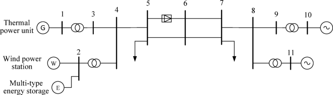
Diagram of the simulation system.

Table 1 Simulation system parameters.

Utilizing operational data from wind power stations located in Qinghai, 3650 sets of system disturbance data samples are generated prior to implementing the DPGMM-LSTM optimization solution. These samples are partitioned into an offline training set and a test verification set in a 6:4 ratio (2190:1460). Furthermore, the DPGMM-LSTM model comprises 4 LSTM layers within its hidden layers, with the network architecture detailed in Table 2. The output layer is a Dense fully connected layer. The learning rate for the neurons within the DPGMM-LSTM network is set at 0.01, and a random dropout rate of 0.35 is applied to the training data.

Table 2 Network parameters.

Validation of the DPGMM-LSTM-Based optimization model solution

In the simulation, a DC unipolar blocking fault is simulated on line 5–6 of the system, resulting in a loss of 1000 MW of active power. The trained DPGMM-LSTM network is then employed to assess and validate the frequency response variations of the sending-end power system, as shown in Fig. 7.

As shown in Fig. 7, after the fault disturbance, the system frequency variation curve derived from the DPGMM-LSTM network closely mirrors that of the actual data samples. Although there are minor discrepancies at certain points, the overall error remains minimal. Furthermore, the performance of the DPGMM-LSTM network is evaluated using evaluation index, with the results presented in Table 3. The results indicate that the DPGMM-LSTM network demonstrates the terms of solution accuracy.

Fig. 7

Frequency response changes of the sending-end power system.

Table 3 Performance evaluation of DPGMM-LSTM solving network.

Examination of system frequency fluctuations with varying frequency regulation parameters

The behavior of the system frequency under varying frequency regulation control parameters is evaluated across three dimensions: the different frequency regulation output ratios of MFRRR, the different frequency additional control proportional coefficients of BSSs, and the different droop coefficients of IELs. The simulation maintains the premise of a DC unipolar blocking fault on line 5–6, resulting in a 1000 MW active power loss.

(1) Different Frequency Regulation Output Ratios of MFRRR.

The frequency regulation output ratio for MTES is fixed at 0.25, for IELs at 0.05, and for WTs and TPUs collectively at 0.7. Other parameters are configured as per Table 1. The simulation and analysis of the frequency variation in the sending-end power system, under these varying output ratios, are conducted. The results are presented in Table 4; Fig. 8.

Table 4 System frequency deviation under different frequency regulation output ratios.

Fig. 8

System frequency changes under different frequency regulation output ratios.

Based on the data presented in Table 4; Fig. 8, it is observed that when implementing the coordinated optimization strategy for frequency regulation reserves, the recovery speed and the final stable state of the frequency change with different frequency regulation output ratios for WTs and TPUs. On the one hand, as the frequency regulation output ratio of WTs reduces from 0.6 to 0.1, the steady-state system frequency deviation gradually decreases. This indicates that a smaller the frequency regulation output of WTs during primary frequency regulation results in a lesser impact on the steady-state system frequency deviation. On the other hand, as the frequency regulation output ratio of WTs decreases from 0.6 to 0.1, the system frequency deviation recovery slows, with the deviation dropping from 0.00227 Hz to 0.00057 Hz. This indicates that a higher frequency regulation output ratio for WTs aids in a quicker system frequency recovery.

(2) Different Frequency Additional Control Proportional Coefficients of BSSs.

The frequency regulation output ratios for WTs, MTES, IELs, and TPUs are set at 0.4, 0.25, 0.05, and 0.3, respectively. Additionally, ${K_{{\text{EES}}}}$ is varied to 5, 10, 15, and 20, with other parameters following Table 1. The simulation and analysis of the frequency changes in the sending-end power system under these varying coefficients are conducted. The results are detailed in Table 5; Fig. 9.

Table 5 System frequency deviation under different ${K_{{\text{EES}}}}$.

Fig. 9

System frequency changes under different ${K_{{\text{EES}}}}$.

Analysis of the data presented in Table 5; Fig. 9 reveals the capacity of the frequency regulation reserve optimization strategy to bolster the resilience of power systems. With an increment in the frequency additional control proportional coefficients of BSSs from 5 to 20, there is a progressive reduction in the absolute value of the system frequency deviation of the steady-state system, an escalation in the maximum system frequency deviation, and a quicker return to the minimum deviation. This indicates that a higher frequency additional control proportional coefficient in BSSs facilitates a swifter recovery of frequency deviation in the sending-end power system and contributes to a more stable frequency equilibrium.

(3) Different Droop Coefficients of IELs.

The frequency regulation output ratios for WTs, MTES, IELs, and TPUs are adjusted to 0.3, 0.25, 0.2, and 0.25, respectively. ${\kappa _{{\text{Load}}}}$ is sequentially set to 4, 8, 12, and 16, with other parameters following the specifications in Table 1. The simulation and analysis of the sending-end power system’s frequency fluctuations under these varying IEL droop coefficients are conducted, with results detailed in Table 6; Fig. 10.

The results from Table 6; Fig. 10 indicate that under the frequency regulation reserve optimization strategy, and with constant frequency regulation output ratios for WTs, MTES, IELs, and TPUs, the steady-state system frequency deviation of the sending-end power system rises from − 0.2417 Hz to -0.1983 Hz as the droop coefficient ${\kappa _{{\text{Load}}}}$ increases from 4 to 16. Additionally, the peak frequency deviation during the system frequency drop increases from − 0.4450 Hz to -0.3266 Hz. This indicates that an elevated droop coefficient for IELs aids in achieving greater frequency stability in the sending-end power system, with a reduced absolute value of steady-state frequency deviation.

Table 6 System frequency deviation under different ${\kappa _{{\text{Load}}}}$.

Fig. 10

System frequency changes under different ${\kappa _{{\text{Load}}}}$.

Validation of the system frequency regulation reserve cost optimization strategy with MFRRR access

To further verify the efficacy of the frequency regulation reserve cost optimization for MFRRR, it is assumed that a DC unipolar blocking fault occurs on line 5–6 of the simulation system, resulting in a loss of 1500 MW of active power. The parameters are configured in accordance with Table 1. Concurrently, three distinct scenarios for power system frequency regulation reserve optimization are established for comparative analysis, allowing for a comprehensive evaluation of the strategy’s performance under various conditions.

Scenario 1: Only consider thermal power units as MFRRR for system frequency regulation.

Scenario 2: Only consider wind turbines as frequency regulation reserves for system frequency regulation.

Scenario 3: Consider wind turbines, multi-type energy storage, integrated energy loads, and thermal power units as MFRRR for system frequency regulation. This is the frequency regulation reserve cost optimization method in this paper.

The three scenarios are solved by the DPGMM-LSTM solution network proposed in this paper. The frequency deviation of the sending-end power system under the three scenarios are shown in Fig. 11; Table 7. The output results of frequency regulation reserve resources in three scenarios are shown in Fig. 12.

Fig. 11

System frequency changes under three schemes.

Table 7 Network parameters.

Fig. 12

Reserve output.

Based on the results, it can be seen that the frequency deviation of the sending-end power system under the Scenario 1 changes greatly, and the system frequency recovery time is longer. Under the Scenario 2, when the WTs are used as the MFRRR and have a high rated capacity, it can provide more frequency regulation reserve capacity when participating in the primary frequency regulation, reducing the absolute value of the system frequency deviation. Furthermore, under the Scenario 3, the collaborative adjustments of wind power units, MTES, IELs, and TPUs are used to improve the overall frequency regulation reserve capacity of the system, thereby reducing the absolute value of system frequency deviation. From the perspective of frequency regulation reserve cost, the frequency regulation reserve cost of the Scenario 3 is the best. Therefore, the frequency regulation reserve cost optimization method proposed in this paper can effectively improve the frequency stability and frequency regulation economy of the power system.

Conclusion

An optimization approach for the frequency regulation reserve costs in wind power stations is proposed, focusing on the cooperative involvement of multi-frequency regulation reserve resources (MFRRR) in power system frequency regulation. The following conclusions are as follows:

• (1) A model depicting the frequency regulation characteristics of MFRRR within wind power stations engaged in power system frequency regulation has been developed. This model facilitates the analysis of the frequency response regulation processes of wind turbines, multi-type energy storage systems, integrated energy loads, and thermal power units. It enables the coordinated response of MFRRR to system frequency fluctuations.

• (2) An optimization model for the frequency regulation reserve costs of MFRRR in wind power stations has been established. This model is capable of mitigating system frequency deviations by dynamically adjusting the output of each reserve resource upon system disturbances. It ensures the stability of system frequency and enhances the economic viability of wind power stations in their primary frequency regulation role within the power system.

In future research, the research will focus on improving the accuracy and adaptability of the model, introducing advanced machine learning methods to optimize the architecture and parameters of the DPGMM-LSTM model, and enhancing the fitting and generalization ability of the DPGMM-LSTM model for complex working conditions. At the same time, multi-source data fusion analysis of multi-frequency regulation reserve resources of wind farm stations is carried out to integrate multi-dimensional data resources of wind farms, so as to grasp the key information in the frequency regulation process more comprehensively and provide more abundant data support for model optimization and strategy formulation. In addition, in-depth analysis of various economic factors in the process of frequency modulation, including maintenance costs and market trading mechanisms, will be conducted to build a more comprehensive and accurate economic analysis model and provide more valuable reference for practical applications.

References

Teng, Y., Zhang, T. & Chen, Z. Review of operation optimization and control of multi-energy interconnection system based on microgrid. Renew. Energy. 36 (03), 467–474 (2018).
Shen, W. et al. Low-carbon electricity network transition considering retirement of aging coal generators. IEEE Trans. Power Syst. 35 (6), 4193–4205. https://doi.org/10.1109/TPWRS.2020.2995753 (2022).
Liu, S. et al. Voltage optimal control model of regional distribution network after reconfiguration based on multi-energy conversion. Electr. Power Syst. Res. 37, 110994 (2024). https://doi.org/j.epsr.2024.110994
Mirmohammad, M. & Azad, S. P. Control and stability of Grid-Forming inverters: a comprehensive review. Energies. 17(13), 3186 (2024). https://doi.org/10.3390/en17133186
Wang, X. et al. Grid-synchronization stability of converter-based resources: an overview. IEEE Open. J. Ind. Appl. 1, 115–134. https://doi.org/10.1109/OJIA.2020.3020392 (2020).
Zhao, M. et al. Optimal coordinated frequency regulation of renewable energy systems via an equilibrium optimizer. Front. Energy Res. 10, 950524. https://doi.org/10.3389/fenrg.2022.950524 (2022).
Cai, S., et al. Frequency characteristics of southwest power grid and scheme of over-frequency generator tripping. 2021 IEEE IAS Industrial and Commercial Power System Asia (IEEE I&CPS ASIA 2021), 1017–1022. https://doi.org/10.1109/ICPSAsia52756.2021.9621515 (2021).
Xue, J. et al. Transient frequency stability emergency control for the power system interconnected with offshore wind power through VSC-HVDC. IEEE Access. 8, 53133–53140. https://doi.org/10.1109/ACCESS.2020.2981614 (2020).
Liu, D., Zhang, X. & Tse, C. Effects of high level of penetration of renewable energy sources on cascading failure of modern power systems. IEEE J. Emerg. Sel. Top. Circuits Syst. 12 (1), 98–106. https://doi.org/10.1109/JETCAS.2022.3147487 (2022).
Yan, X. et al. Study of inertia and damping characteristics of doubly fed induction generators and improved additional frequency control strategy. Energies 12 (1), 38. https://doi.org/10.3390/en12010038 (2019).
Shi, Q. et al. Coordinated virtual inertia control strategy for D-PMSG considering frequency regulation ability. J. Electr. Eng. Technol. 11 (6), 1556–1570. https://doi.org/10.5370/JEET.2016.11.6.1556 (2016).
Hu, Y. & Wu, Y. Approximation to frequency control capability of a DFIG-based wind farm using a simple linear gain droop control. IEEE Trans. Ind. Appl. 55 (3), 2300–2309. https://doi.org/10.1109/TIA.2018.2886993 (2019).
Zhao, F. et al. Comparative study of battery-based STATCOM in grid-following and grid-forming modes for stabilization of offshore wind power plant. Electric Power Syst. Res. 212 108449. https://doi.org/10.1016/j.epsr.2022.108449
Narula, A. et al. Empowering offshore wind with ES-STATCOM for stability margin improvement and provision of grid-forming capabilities. Electric Power Syst. Res. 234, 110801. https://doi.org/10.1016/j.epsr.2024.110801 (2024).
He, Y. et al. Investigation on grid-following and grid-forming control schemes of cascaded hybrid converter for wind power integrated with weak grids. Int. J. Electr. Power Energy Syst. 155 (8), 109524. https://doi.org/10.1016/j.ijepes.2023.109524 (2024).
Qi, J. et al. Research on frequency response modeling and frequency modulation parameters of the power system highly penetrated by wind power. Sustainability 14 (13), 7798. https://doi.org/10.3390/su14137798 (2022).
Yang, P. et al. Coordinated control of rotor kinetic energy and pitch angle for large-scale doubly fed induction generators participating in system primary frequency regulation. IET Renew. Power Gener. 15 (8), 1836–1847. https://doi.org/10.1049/rpg2.12153 (2021).
Jia, Y. et al. Control strategy of flywheel energy storage system based on primary frequency modulation of wind power. Energies 15 (5), 1850. https://doi.org/10.3390/en15051850 (2022).
Sun, M. et al. Optimal auxiliary frequency control of wind turbine generators and coordination with synchronous generators. CSEE J. Power Energy Syst. 7 (1), 78–85. https://doi.org/10.17775/CSEEJPES.2020.00860 (2021).
Zhang, H. et al. Frequency-constrained expansion planning for wind and photovoltaic power in wind-photovoltaic-hydro-thermal multi-power system. Appl. Energy. 356, 122401. https://doi.org/10.1016/j.apenergy.2023.122401 (2024).
Jung, J., Kim, S. & Kim, H. Spatially-correlated time series clustering using location-dependent dirichlet process mixture model. Stat. Anal. Data Min. 17 (1). https://doi.org/10.1002/sam.11649 (2024).
Lei, S. et al. Research on a LSTM based method of forecasting primary frequency modulation of grid. J. Internet Technol. 21 (3), 791–798. https://doi.org/10.3966/160792642020052103016 (2020).
Li, P. et al. The integrated control strategy for primary frequency control of DFIGs based on virtual inertia and pitch control. 2016 IEEE Innovative Smart Grid Technol. - ASIA (ISGT-ASIA). 430–435. https://doi.org/10.1109/ISGT-Asia.2016.7796424 (2017).
Acknowledgements
This work is supported by the “Key Technologies of Optimal Configuration and Integrated Dispatch Control of High-Voltage Direct-Coupled Grid-Forming Energy Storage” (2024ZD0800200).
Author information
Authors and Affiliations
Contributions
Han Zhang: Conceptualization, methodology, formal analysis, writing - original draft preparation, funding acquisition, and project administration.Maoyuan Zhang, Xin Li, and Chunwei Song: Data curation, investigation, validation, and writing - review and editing.All authors have read and agreed to the published version of the manuscript.
Corresponding author
Ethics declarations
Competing interests
The authors declare no competing interests.
Additional information
Publisher’s note
Springer Nature remains neutral with regard to jurisdictional claims in published maps and institutional affiliations.
Rights and permissions
Open Access This article is licensed under a Creative Commons Attribution-NonCommercial-NoDerivatives 4.0 International License, which permits any non-commercial use, sharing, distribution and reproduction in any medium or format, as long as you give appropriate credit to the original author(s) and the source, provide a link to the Creative Commons licence, and indicate if you modified the licensed material. You do not have permission under this licence to share adapted material derived from this article or parts of it. The images or other third party material in this article are included in the article’s Creative Commons licence, unless indicated otherwise in a credit line to the material. If material is not included in the article’s Creative Commons licence and your intended use is not permitted by statutory regulation or exceeds the permitted use, you will need to obtain permission directly from the copyright holder. To view a copy of this licence, visit http://creativecommons.org/licenses/by-nc-nd/4.0/.
About this article
Cite this article
Zhang, H., Zhang, M., Li, X. et al. Reserve optimization model of wind power with the coordination of multiple type electric power system sources. Sci Rep 15, 27663 (2025). https://doi.org/10.1038/s41598-025-12887-7
Received:
Accepted:
Published:
Version of record:
DOI: https://doi.org/10.1038/s41598-025-12887-7