Optimization of roof slope, design and wood strength classes in timber Fink type truss

Abstract

Wood is widely used in structural systems worldwide due to its mechanical properties and sustainability. In Brazil, its application is relative modest compared to Northern Hemisphere countries yet remains prevalent in roof structures, some of which date back to the twentieth century. Over time, empirical assumptions have influenced the design of timber roof structures has been observed, such as those related to roof slope. Many builders assume that lower slopes reduce material consumption since shorter elements are required. However, the magnitude of forces on the members is inversely proportional to the slope, potentially resulting in oversized structures. To assess the validity of these assumptions, this study investigates the optimal slope and appropriate strength class for a Fink truss with a 10-m span, employing the Firefly Algorithm for optimization. The results indicate that the D20 strength class, which has a characteristic compressive strength of 20 MPa, was optimal, reducing timber volume by up to 32.4% compared to higher strength classes, which significantly decreases structural mass and column loads. Specifically, optimal slopes ranged between 10° and 15°, achieving a total timber volume below 0.20 m3. It was observed that lower slopes (e.g., 5°) increased material volume by up to 324%, compared to the optimal slope configuration (typically between 10° and 15°), primarily due to strength and stability requirements. Similarly, very high slopes (above 36°) led to an average volume increase of approximately 250%. Furthermore, adopting a cross-sectional dimensions of 75 × 75 mm provided an effective solution to control slenderness within regulatory limits, ensuring both structural efficiency and economical usage of timber.

Introduction

Wood, a sustainable and renewable material, meets key criteria to be used in structural applications¹. It has been utilized in construction for centuries², providing both functionality and aesthetic appeal³. Compared to other structural materials such as concrete and steel, wood exhibits several advantages, particularly with three main highlights:

• Low energy consumption in production: Steel, refined petroleum products, and chemical industries account for approximately 80% of the world’s energy is consumed by steel, refined petroleum products, and chemical producers⁴. Cement production, a critical component of concrete, requires vast amount of coal and releases substantial CO₂ into the atmosphere⁵. Conversely, wood not only demands less energy in its processing^6,7 but actively sequesters CO₂, as trees absorb this gas during photosynthesis for oxygen release⁸.

• Renewable and environmentally friendly: Wood is a sustainable, recyclable material² that has a significantly lower environmental impact than conventional structural materials⁹. The optimized use of wood products enhances the sustainability of the forest-wood supply chain and contributes to climate change mitigation^10,11.

• High strength-to-weight ratio: In tension, softwoods can have a strength-to-weight ratio approximately two times higher than structural steel¹². In compression, the same ratio is approximately six times higher than concrete¹². As for hardwoods, in tension, this magnitude is approximately three times greater than that of steel, and in compression, it can reach up to ten times that of concrete¹³.

Significant advancements in wood-derived products, particularly those sourced from planted forests, have been observed in recent years¹⁴. This has driven interest in a consumer market that prioritizes environmentally friendly products. Notably, wood remains a key material in modern infrastructure projects worldwide, including bridges, railway infrastructure, among many others^15,16.

Wood’s high strength-to-weight ratio makes it particularly suitable for roofing structures, a topic frequently explored in scientific research^17,18. In Brazil, although its usage is less prevalent than in Northern Hemisphere countries, wood remains a widely adopted material in various structural applications, particularly for roofs. The country has developed impressive structures with large spans, such as sports arenas, hangars, and rural warehouses. Remarkably, some of these structures, built throughout the twentieth century, remain intact today, demonstrating that proper maintenance and treatment can ensure long-term durability^19,20.

However, over time, certain empirical assumptions have influenced the design of wooden roof structures. One such assumptions concerns the slope between the truss chords, where builders often believe that smaller slopes reduce material consumption due to shorter member lengths^21,22. In reality, lower slopes result in higher applied forces, ultimately increasing material demands^22,23. Moreover, real-world truss design involves multiple considerations beyond structural efficiency, such as investor preferences, building regulations, transportation costs, and intended building use. These factors introduce additional complexities, with their significance varying depending on project requirements. For example, while economic factors may favor standardized construction techniques, architectural or functional demands might prioritize aesthetics and space utilization over pure material efficiency. Therefore, this study’s recommended roof slope should be seen as a guideline rather than a fixed rule, allowing for adjustments based on broader design considerations. Even with wood’s recognized environmental benefits, adopting a rational design approach is essential to prevent material waste and optimize resource management.

Some researchers have investigated this variable^22,23. In studies examining slopes ranging from 5° to 15° in Pratt and Howe trusses with 10-m spans, results showed that a 15° slope resulted in the lowest material consumption^22,23. However, these studies simplified their analyses by keeping the member thickness constant and varying only the height. As a result, they focused solely on the impact of the slope on member design, without determining the optimal design slope. Additionally, these studies exclusively considered a single hardwood strength class.

To address these limitations, this study expands the scope beyond prior research, such as that of Fraga et al.²² and Menezes et al.²³. Earlier studies restricted their analysis to a narrow range of roof slopes (5°–15°), employed simplified manual calculation methods, and focused exclusively on a single wood strength class. Moreover, they did not account for essential design factors such as member slenderness and stability. This study overcomes these constraints by extending the slope range to 41° and incorporating an automated optimization process using the Firefly Algorithm (FA). Additionally, it evaluates multiple strength classes (D20–D60), significantly enhancing the flexibility of wood selection. Stability and slenderness, critical factors often overlooked in previous research, are systematically analyzed, reinforcing this study’s contribution toward more sustainable, structurally efficient, and cost-effective timber truss designs.

To achieve these objectives, this study employs a robust optimization methodology based on the FA. Pereira et al.²⁴ demonstrated that the FA achieves rapid convergence, stable outcomes, and minimal variation compared to alternative optimization methods such as Genetic Algorithms (GA), Particle Swarm Optimization (PSO), and Simulated Annealing (SA). Furthermore, the FA’s ability to handle discrete design variables, including standard timber cross-sections, strengthens its suitability for this study. The research examines a broad range of roof slopes (5° to 41°) and five strength classes (D20; D30; D40; D50; D60) as stipulated in the Brazilian normative document ABNT NBR 7190-1²⁵, which has recently undergone updates. While primarily based on the Brazilian standard, the methodology and results align significantly with international standards such as Eurocode 5, particularly regarding design criteria and verification of structural elements, thereby enhancing the global applicability and relevance of the findings.

In this way, the results presented in this study will significantly contribute to promoting the more efficient utilization of wood in roofing structures.

Material and methods

In this section, information regarding the study object will be addressed, namely, a timber truss roof structure, classified by ABNT NBR 8681²⁶ as a type 2 building, with accidental loads not exceeding 5 kN/m².

Geometry

Due to its common geometry of symmetrical gable roofs, the Fink truss typology was adopted. The arrangement of the members depends on the roof slope and the type of roofing material used. In this study, the term ‘slope’ is used to describe the roof slope angle, expressed in degrees, which is equivalent to the term ‘slope’ as commonly used in structural geometry descriptions. Thus, technical catalogs of corrugated fiber cement sheets (commonly used in industrial/rural buildings) were consulted to establish basic guidelines for the design of these geometries²⁷. The first guideline relates to the minimum slope, limited to 5° (9%). In practice, common slopes adopted for Fink-type trusses with corrugated fiber cement roofing systems range between 15° and 30°, based on manufacturer recommendations²⁷. The expanded analysis from 5° to 41° in this study enables evaluation of both typical and boundary configurations, providing a broader understanding of material and structural behavior. It is also important to emphasize a minimum longitudinal overlap between sheets, specified by slope (α) ranges, as printed in Table 1.

Table 1 Minimum longitudinal overlap.

Therefore, the geometries are designed by placing the sheets over the purlins, which are supported by the top chord, while respecting the longitudinal overlaps according to the slope. It is also permissible to have an overhang in the eave region, limited to values greater than 25 cm and less than 40 cm when gutters are not used.

The manufacturer’s catalogs also specify sheet lengths with their respective number of supports. In this study, only corrugated fiber cement sheets with a thickness of 6 mm and lengths of 122 cm, 153 cm, and 183 cm were used, with a minimum number of supports equal to 2.

In determining the position of the purlins located in the ridge region, a complementary ridge piece with a 300 mm flange and a minimum hole distance of 90 mm from its end was considered. For these considerations, the maximum D values given in Table 2 were respected.

Table 2 Maximum distance D between the axes of the purlins located in the ridge region.

In practice, common slopes adopted for Fink-type trusses with corrugated fiber cement roofing systems range between 15° and 30°, based on manufacturer recommendations. The expanded analysis from 5° to 41° in this study enables evaluation of both typical and boundary configurations, providing a broader understanding of material and structural behavior.Following the mentioned guidelines, the configuration of the members and group arrangement are depicted in Fig. 1.

Fig. 1

Configuration of members and group arrangement.

To compare the trusses, the arrangement of the roofing sheets should be such that the number of members remains the same for any given slope. Therefore, starting from the minimum slope of 5° (9%), the maximum slope found was 41° (87%), which requires four sheets of 183 cm in length, a longitudinal overlap of 14 cm, and an approximate free overhang of 33 cm. Table 3 contains the values of longitudinal overlaps and arrangements of sheets used in the design of each geometry.

Table 3 Geometry design parameters.

Loads

The actions and loadings acting on the structure were estimated with the aid of technical catalogs of fiber cement sheets and the ABNT NBR 6120²⁸ and ABNT NBR 6123²⁹ standards.

Dead loads

The dead loads acting on the truss are those arising from the self-weight of the timber structure and the roofing materials. The loading due to self-weight does not need to be inserted in a specific field since the algorithm automatically adapts minimum sections for each group of members, updating the self-weight of the structure at each iteration. The forces due to self-weight (F_j) are distributed to the load application points (joints “j” where the purlins are located). Their estimation is given by Eqs. (1) and (2), where ρ_ap is the apparent density of the wood; A_i is the cross-sectional area of each member; ℓ_i is the linear length of each member; L is the truss span; d_t is the distance between trusses; A_inf,j is the influence area of each joint receiving a purlin, and F_p is the concentrated self-weight of the purlin at the joint:

$${g}_{\text{dead-load}}=\frac{{\rho }_{\text{ap}}\cdot \sum_{i=1}^{n}{A}_{i}\cdot {{\ell}}_{i}}{L\cdot {d}_{t}}$$

(1)

$${F}_{j}=\left({g}_{\text{dead-load}}\cdot {A}_{{\text{inf}},j}\right)+{F}_{p}$$

(2)

Since the self-weight is automatically calculated, the only dead loads considered were those due to the weight of materials fixed to the structure, estimated at approximately 200 N/m² with weight of 6 mm fiber cement sheets ≅ 180 N/m² and sheet metal fittings ≅ 20 N/m².

In the calculation of combinations of actions for the ultimate limit state (ULS), the dead loads were considered separately. For this situation, the load weighting coefficients (γ) printed in Table 4 were assumed, taken from item 6.1 of ABNT NBR 7190-1²⁵ and Table 1 of ABNT NBR 8681²⁶. It is worth mentioning that unfavorable effects occur when the dead loads act in the same direction as the main live load, while favorable effects occur in the opposite direction to the main live load.

Table 4 Weighting coefficients for dead loads.

Live load and wind load

The minimum live loads acting on roof structures are the accidental load and wind load. The accidental load corresponds to the minimum value of 250 N/m² in horizontal projection, as recommended by item 6.4 of ABNT NBR 6120²⁸ for slopes equal to or greater than 3% (1.7°).

The wind action on the structure was quantified following the normative recommendations of ABNT NBR 6123²⁹, considering a rectangular building with a symmetrical gable roof. Figure 2 illustrates the floor plan, the cross-section, and the scheme of openings adopted for the building.

Fig. 2

Floor plan and cross-section of building (dimensions in meters).

From Fig. 2, it can be observed that all dimensions of the building are fixed, except for the height of the roof (h), which varies according to the truss slope. Since the wind action on the building also varies with the height of the roof, to simplify the application of loads, it was decided to select the critical wind action among the 37 analyzed slopes. According to the ABNT NBR 6123²⁹, for a ratio between wall height and building width equal to or less than 0.5, the slope of 10° corresponds to the critical situation. Table 5 presents the parameters used in the calculation of the dynamic wind pressure for the slope of 10°, with a roof height equal to 0.882 m.

Table 5 Parameters for calculating dynamic wind pressure (q).

Therefore, the final dynamic pressures (q) are given by Eq. (3):

$$q = 0.613 \cdot v_{k}^{2} \Rightarrow \left\{ {\begin{array}{*{20}c} {0^\circ \,{\text{wind:}}\,\, 0.613 \cdot 33.25^{2} = 678 \,{\text{N}}/{\text{m}}^{2} } \\ {90^\circ \,{\text{wind:}}\,\, 0.613 \cdot 32.47^{2} = 646 \,{\text{N}}/{\text{m}}^{2} } \\ \end{array} } \right.$$

(3)

To quantify the wind action on the building, pressure was combined with the external and internal pressure coefficients. The external pressure coefficients (C_e) on the roof were determined using Table 7 of ABNT NBR 6123²⁹, considering the critical roof slope (10°) and the ratio between the wall height and the building width equal to 0.4. The values are illustrated in Fig. 3.

Fig. 3

External shapes coefficients.

The internal pressure coefficients were quantified based on assumptions of dominant openings in different regions of the building (Fig. 2). For this purpose, fixed openings of 10 cm were considered on each face of the building, along with a 5 cm gap below the indicated gate in Fig. 2. Table 6 presents the internal pressure coefficients (c_pi) for the critical assumptions prescribed in item 6.3.2 of ABNT NBR 6123²⁹. It should be emphasized that the objective was to extract the critical case of suction, which occurred at a wind angle of 90°, and the critical case of overpressure, which occurred at a wind angle of 0°.

Table 6 Values of internal pressure coefficients.

Finally, the calculated value of the wind action on the building (w_k) is shown in Eq. (4).

$$w_{k} = \left( {C_{e} - c_{pi} } \right) \cdot q \Rightarrow \left\{ {\begin{array}{*{20}l} {0^\circ \,{\text{wind:}}\,\, \left( { - 0.2 + 0.805} \right) \cdot 678 \cong 410\,{\text{N}}/{\text{m}}^{2} } \hfill \\ {90^\circ \,{\text{wind:}}\,\, \left( { - 1.2 - 0.690} \right) \cdot 646 \cong - 1220\,{\text{N}}/{\text{m}}^{2} } \hfill \\ \end{array} } \right.$$

(4)

In the ULS and serviceability limit states (SLS), the live load and wind load were considered separately, assuming the coefficients printed in Table 7, extracted from Tables 4 and 6 of ABNT NBR 8681²⁶.

Table 7 Weighting (γ) and reduction (ψ) coefficients for live load and wind load.

Structural analysis and load combinations

Using the finite element method (FEM), the structural analysis model employed in the processing of the structure was that of a classical truss, i.e., perfectly hinged bar elements at their ends and subjected only to axial forces. Figure 4 illustrates the static scheme employed in all simulations.

Fig. 4

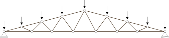
Static scheme of classic truss model.

The soliciting forces produced by each load described in section “Loads” need to be combined with each other to generate critical values for structural design. Using the weighting (γ) and reduction (ψ) coefficients, the design soliciting forces were obtained according to expressions from ABNT NBR 7190-1²⁵ for ULS under normal conditions, as transcribed in Eq. (5) below.

$${F}_{d}=\sum_{i=1}^{m}{\gamma }_{gi}\cdot {F}_{Gi,k}+{\gamma }_{q1}\cdot {F}_{Q1,k}+\sum_{j=2}^{n}{\gamma }_{qj}\cdot {\psi }_{0,j}\cdot {F}_{Qj,k}$$

(5)

Table 8 contains the three critical load combinations considered. The variable F in the second column of Table 8 corresponds to the characteristic design force due to the following factors: SW—self-weight; SH—roof sheets; AC—accidental loads; WD,o—wind overpressure; WD,s—wind suction.

Table 8 Critical load combinations (ULS)—normal conditions.

It should be noted that the live actions (accidental and suction wind) are not grouped in F_d,3, as they are of opposite nature and have divergent directions, which does not lead to critical values of soliciting forces when summed in the same equation. Attention is also drawn to the 25% reduction in the forces resulting from wind action in F_d,3. The multiplication by 0.75 is in accordance with the recommendation of item 6.1 of ABNT NBR 7190-1²⁵, which considers the high strength of wood under short-duration loads when they represent the main variable action in isolation.

On the other hand, the combinations for SLS regarding structural deformations were calculated according to Eqs. (6) and (7), extracted from ABNT NBR 7190-1²⁵ corresponding to the long-duration class. In Eqs. (6) and (7), δ_inst represents instantaneous displacements, δ_fin represents final displacements, considering the effects of creep, and ϕ is the creep coefficient of wood, equal to 0.6 for sawn timber exposed to moisture class 1 (U_amb ≤ 65%).

$${\delta }_{\text{inst}}=\sum_{i=1}^{m}{\delta }_{{\text{inst}},Gi,k}+{\delta }_{{\text{inst}},Q1,k}+\sum_{j=2}^{n}{{\psi }_{1,j}\cdot \delta }_{{\text{inst}},Qj,k}$$

(6)

$${\delta }_{\text{fin}}=\sum_{i=1}^{m}{\delta }_{{\text{inst}},Gi,k}\cdot \left(1+\phi \right)+\sum_{j=1}^{n}{\delta }_{{\text{inst}},Qj,k}{\cdot \psi }_{2,j}\cdot \left(1+\phi \right)$$

(7)

Table 9 contains the four critical displacements combinations considered. The variable δ_inst in the second column of Table 9 corresponds to the instantaneous displacements to the following factors: SW—self-weight; SH—roof sheets; AC—accidental loads; WD,o—wind overpressure; WD,s—wind suction.

Table 9 Critical load combinations (ULS)—normal conditions.

It is observed that the displacements resulting from wind action are disregarded in δ_fin because they are of short duration and do not affect the long-term normal use of the structure.

Design

Based on the calculated forces and displacements, the parameters for structural design followed the recommendations of ABNT NBR 7190-1²⁵, it is worth highlighting that the Brazilian standard was strongly inspired by Eurocode 5³⁰.

Strength classes, modification factors and purlin dimensions

For the components that will make up the roof purlins, the adopted wood species belongs to the Hardwoods group, class D40, defined in tests conducted on defect-free specimens. The characteristic values of compressive strength parallel to the grain (f_c0,k), shear strength parallel to the grain (f_v0,k), mean value of the modulus of elasticity in compression parallel to the grain (E_c0,m), and apparent density at 12% moisture content (ρ_ap) were extracted from Table 2 of ABNT NBR 7190-1²⁵ and presented in Table 10.

Table 10 Hardwood’s strength classes (Values in standard reference condition U = 12%).

Regarding the truss members, the processing of the four strength classes within the hardwoods group was chosen to obtain the optimal strength class along with the corresponding slope. Table 10 presents the values of strength, stiffness, and apparent density for each class within the hardwoods group.

According to the recommendations of ABNT NBR 7190-1²⁵, in the absence of characterization of tensile strength parallel to the grain (f_t0,k) and bending strength (f_b,k), it was assumed that f_t0,k = f_b,k = f_c0,k.

The modification coefficients (k_mod) were quantified based on the standard, varying according to the loading class, wood processing type, and moisture class. In this study, two live loads were estimated, with different loading classes: long-duration for accidental load and short-duration for wind load. To facilitate the estimation of the partial coefficient k_mod,1 in all combinations, a long-duration loading was assumed, while the short-duration action (wind) was multiplied by 0.75 when it was the primary action in the combination, already included in F_d,3, Table 8. Therefore, assuming lumber exposed to an environment with relative humidity equal to or less than 65% (moisture class 1), the final modification coefficient (k_mod) assumes a value of 0.70.

Prior to the truss design process, it is necessary to determine the sections that will compose the purlins. Although they are part of the self-weight of the wooden structure, they must be designed before the truss so that their actual loading is predicted and applied properly to the joints where they are located. These elements were treated as simply supported beams subjected to oblique bending, with a theoretical span equal to the distance between the trusses, limited to 3.0 m.

After the design process, it was found that a section of 60 × 120 mm meets all the verifications. Therefore, its self-weight is approximately 162 N (see Eq. (8)). Thus, at each joint where a purlin is located, a point load of 162 N was applied. It is worth noting that there are two purlins at the ridge joint, resulting in a value of 324 N at that location.

$${F}_{\text{purlin}}={\rho }_{ap}\cdot V=750\cdot \left(0.06\cdot 0.12\cdot 3.0\right)=16.2\,{\text{kg}}\cong 162\, {\text{N}}$$

(8)

Design standard for truss structures

The members that make up the truss structures are considered to have a full rectangular cross-section, as depicted in Fig. 5, where t, h, and L₀ represent the thickness, height, and linear length, respectively.

Fig. 5

Geometric representation and arbitrated variables for the member dimensions.

The cross-sectional area (A_i), slenderness ratio (λ_i), and radius of gyration (r_i) of a generic member i are expressed by Eqs. (9), (10), and (11) respectively. Here, ${t}_{i}$ and ${h}_{i}$ correspond to the thickness and height of the member’s cross-section, respectively, and ${L}_{0,i}$ is the linear length of the member. ${I}_{i}$ represents the minimum moment of inertia about the critical axis, determined by selecting the dimension (thickness or height) that yields the smallest value. The thickness (${t}_{i}$) directly influences the radius of gyration (${r}_{i}$), thereby affecting the slenderness ratio (${\lambda }_{i}$). A lower slenderness ratio indicates a reduced risk of member buckling under axial compression, essential for ensuring compliance with the stability limits specified by ABNT NBR 7190-1²⁵.

$${A}_{i}={t}_{i}\cdot {h}_{i}$$

(9)

$${\lambda }_{i}={L}_{0,i}/{r}_{i}$$

(10)

$${r}_{i}=\sqrt{{I}_{i}/{A}_{i}}$$

(11)

Considering that the truss members are subjected only to axial forces, i.e., normal to the cross-section, it is of vital importance to verify their stability when subjected to compression, according to the criteria of ABNT NBR 7190-1²⁵. Using the slenderness ratio (λ), limited to values not exceeding 140, and the characteristic value of the modulus of elasticity measured in the direction parallel to the grain (calculated as 70% of E_c0,m), the relative slenderness ratio (λ_rel) in the critical direction is calculated, as per Eq. (12).

$${\lambda }_{\text{rel}}=\left(\lambda /\pi \right)\cdot \sqrt{{f}_{c0,k}/{E}_{\text{0,05}}}$$

(12)

The stability condition for axially compressed members is given by Eq. (13), where σ_Nc,d is the design value of the normal compressive stress on the cross-section, and f_c0,d is the design value of compressive strength parallel to the grain.

$$\frac{{\sigma }_{Nc,d}}{{k}_{c}{\cdot f}_{c0,d}}\le 1.0$$

(13)

The coefficients k_c and k are obtained through Eqs. (14) and (15), respectively, where β_c is the factor for structural members that meet the limits of alignment divergence, equal to 0.2 for lumber.

$${k}_{c}=\frac{1}{k+\sqrt{{k}^{2}-{{\lambda }_{\text{rel}}}^{2}}}$$

(14)

$$k=0.5\cdot \left[1+{\beta }_{c}\cdot \left({\lambda }_{\text{rel}}-0.3\right)+{{\lambda }_{\text{rel}}}^{2}\right]$$

(15)

In addition to stability verification, the safety condition for centrally compressed members is performed according to Eq. (16).

$${\sigma }_{Nc,d}/{f}_{c0,d}\le 1.0$$

(16)

In the design of axially tensioned members, the safety condition established by ABNT NBR 7190-1²⁵ is expressed by Eq. (17), where σ_Nt,d is the design value of normal tensile stress on the cross-section, and f_t0,d is the design value of tensile strength parallel to the grain.

$${\sigma }_{Nt,d}/{f}_{t0,d}\le 1.0$$

(17)

For the design of the truss and the application of design constraints, such as checking the ULS and SLS, it is necessary to obtain the design values of the mechanical properties of wood. As specified in ABNT NBR 7190-1²⁵, the design compressive strength parallel to the grain (f_c0,d) and the effective value of the modulus of elasticity parallel to the grain (E_0,ef) are determined by Eqs. (18) and (19) respectively.

$${f}_{c0,d}={k}_{\text{mod}}\cdot \left({f}_{c0,k}/{\gamma }_{w}\right)$$

(18)

$${E}_{0,{\text{ef}}}={k}_{\text{mod}}\cdot {E}_{c0,m}$$

(19)

where γ_w is the reduction coefficient for wood compressive strength, given a value of 1.4.

Furthermore, all structural failure modes were explicitly considered within the optimization process. The imposed design constraints ensured compliance with slenderness limits and buckling resistance criteria, addressing potential failure mechanisms such as compression buckling, lateral-torsional buckling, and global instability. The slenderness ratio was rigorously controlled according to ABNT NBR 7190-1²⁵, and the optimization algorithm systematically adjusted cross-sectional dimensions to mitigate instability risks. By integrating these considerations, the optimized truss designs achieve a balance between material efficiency and structural robustness, ensuring safe and reliable performance under varying design conditions.

It is worth noting that, in this study, both in-plane and out-of-plane buckling lengths were assumed to be equal to the linear length of each member (${L}_{0}$), as per a conservative 2D modeling approach without intermediate lateral bracing. While this simplification aligns with the design framework adopted by ABNT NBR 7190-1²⁵ and supports standardized member grouping, it may overestimate the risk of buckling in real-world scenarios. In practice, the incorporation of additional structural components—such as lateral bracing or a three-dimensional framework—could significantly reduce the effective buckling lengths, especially for longer compressed members near the ridge. Although such strategies were not considered in the current model, they represent a promising avenue for future research and practical refinement of timber truss designs.

Optimization algorithm

The algorithm used in this study was the Firefly Algorithm (FA), which was proposed by Yang³¹ and can be classified as a bioinspired probabilistic optimization method. This is a population-based method, meaning that more than one particle explores the search space in search of the optimal feasible solution. These methods use the concept of random variables for generating the initial population, which is a random event that respects the problem’s constraints³¹.

The theoretical inspiration for the design of this algorithm was drawn from the phenomenon of bioluminescence and the interactions among fireflies during mating. Therefore, the FA optimization method is based on the ability of fireflies to emit light and the ability of other individuals in the population to perceive this light.

When developing the algorithm, Yang³¹ defined some principles to assist in the development, including:

• All fireflies have a single gender, and being of the same gender, they are attracted to each other.

• The attraction ability of each firefly is proportional to its brightness, which decreases as the distance between individuals in the population increases.

With the generation of initial populations, the firefly (or design variable) starts a random walk, where $\overrightarrow{x}$ moves according to an update function of design variables ($\overrightarrow{\omega }$), as described in Eq. (20), where $\overrightarrow{x}$ is the vector of design variables; $\overrightarrow{\omega }$ is the vector function for updating the design variable, and t is the number of iterations.

$${\overrightarrow{x}}^{t+1}={\overrightarrow{x}}^{t}+{\overrightarrow{\omega }}^{t}$$

(20)

From this new direction, new positions and potential candidate solutions are found to generate the optimal design point³². Thus, the movement between fireflies in the population at each step of the iterative process is given by Eq. (21).

$${\omega }^{t}=\beta \cdot \left({{\overrightarrow{x}}_{j}}^{t}-{{\overrightarrow{x}}_{i}}^{t}\right)+\alpha \cdot \left(\overrightarrow{\eta }-0.5\cdot \overrightarrow{\varepsilon }\right)$$

(21)

where β represents the attractiveness term between fireflies i and j; ${\overrightarrow{x}}_{i}$ represents firefly i; ${\overrightarrow{x}}_{j}$ represents firefly j; $\overrightarrow{\eta }$ is the vector of random numbers between 0 and 1; α is the randomness factor, and $\overrightarrow{\varepsilon }$ is a unit vector.

The randomness factor α follows an exponential decay behavior based on the number of iterations t, following the formulation proposed in Eq. (22), where θ is the decay constant with a value of 0.98.

$$\alpha ={\alpha }_{\text{min}}+\left({\alpha }_{\text{max}}-{\alpha }_{\text{min}}\right)\cdot {\theta }^{t}$$

(22)

As mentioned, the term β represents the attractiveness between fireflies in the swarm. This attractiveness is described according to Eq. (23), where β₀ is the attractiveness for a distance r = 0; r_ij is the Euclidean distance between fireflies i and j, Eq. (24), and γ is the light absorption parameter (Eq. (25)).

$$\beta ={\beta }_{0}\cdot {\text{exp}}\left(-\gamma \cdot {{r}_{ij}}^{2}\right)\approx \frac{{\beta }_{0}}{1+\gamma \cdot {{r}_{ij}}^{2}}$$

(23)

$${r}_{ij}=\Vert {\overrightarrow{x}}_{i}-{\overrightarrow{x}}_{j}\Vert =\sqrt{\sum_{k=1}^{d}{\left({\overrightarrow{x}}_{i,k}-{\overrightarrow{x}}_{j,k}\right)}^{2}}$$

(24)

$$\gamma =\frac{1}{{\left({x}_{\text{max}}-{x}_{\text{min}}\right)}^{2}}$$

(25)

where k represents the k-th component of the design variable vector $\overrightarrow{x}$; d is the number of design variables; x_max is the upper limit of the design variables, and x_min is the lower limit of the design variables.

The application of the FA or any other population-based probabilistic optimization method requires attention to the definition of algorithm parameters (attractiveness: β and γ; randomness: α).

The parameter γ characterizes the variation of attractiveness {γ ∈ [0, ∞)}, and its value is crucially important in determining the convergence speed and behavior of the algorithm. For most applications, this value ranges between 0.10 and 10³¹.

The pseudocode for the FA can be written following the structure presented in Fig. 6.

Fig. 6

Pseudocode of Firefly Algorithm.

The Firefly Algorithm was selected for this study due to its proven effectiveness in handling constrained optimization problems with discrete variables, such as the selection of strength classes and sectional dimensions in timber trusses. Additionally, its search mechanism based on attractiveness and stochastic movement makes it suitable for global design space exploration under structural constraints. This choice is supported by Wang³³, who conducted a comprehensive comparative study involving eleven popular metaheuristic algorithms, and demonstrated that the Firefly Algorithm achieves competitive results in terms of accuracy, stability, and convergence across diverse benchmark functions. While a direct comparison with alternative metaheuristics is not presented in this paper, we acknowledge that such analysis could complement this work and represent a valuable extension for future studies.

Handling constraints

In optimization problems applied to engineering, the use of constraints is necessary as they define the search space for the design variables³⁴. The evaluation of constraints can be approached in two ways: indirect (or classical) and direct. In this study, the indirect or classical approach was adopted, which involves transforming a constrained optimization problem into an unconstrained optimization problem³⁵.

In this research, the method of static exterior penalty was employed, which imposes penalty criteria. The criteria are based on evaluating the population with respect to the constraints, where a penalty function is applied to the solutions that violate the constraints. The exterior penalty coefficient R_p is used to activate this penalty. The complete pseudo-objective problem (penalized objective function) is expressed by Eq. (26).

$$W\left(\overrightarrow{x}\right)=FO\left(\overrightarrow{x}\right)+\sum_{j=1}^{m}{R}_{p}\cdot {{\text{max}}\left[0, {g}_{j}\left(\overrightarrow{x}\right)\right]}^{2}+\sum_{k=1}^{n}{R}_{p}\cdot {\left[{h}_{k}\left(\overrightarrow{x}\right)\right]}^{2}$$

(26)

In Eq. (26), (j, k) represents the j-th inequality constraint and k-th equality constraint, respectively; (m, n) are the total number of inequality and equality constraints, respectively; $\overrightarrow{x}$ is the solution vector (random population); g and h are the set of inequality and equality constraints, respectively; and W($\overrightarrow{x}$) is the penalized objective function.

Optimization algorithm parameters

Table 11 presents the input parameters of the FA based on the study by Pereira et al.²⁴. In this research, a total population of 15 individuals will be considered, generated randomly. A total of 500 generations will be employed.

Table 11 FA Input Parameters.

Objective function

The optimization problem aims to minimize the total weight of the structural system while considering constraints on joint displacements, mechanical strength of the members, and geometric criteria that may cause lateral instability in the structural system. The objective function of the system is expressed by Eq. (27), where A_i is the cross-sectional area of member i, ρ_i is the material density, L_0,i is the length of member i in the truss, and n is the number of members in the truss.

$$FO\left({A}_{i},{\rho }_{i},{L}_{0,i}\right)=\sum_{i=1}^{n}{A}_{i}\cdot {\rho }_{i}\cdot {L}_{0,i}$$

(27)

As mentioned, the exterior penalty technique^34,36 was employed to handle the constrained optimization problem. In this technique, the objective function is modified to become a pseudo-objective function, where g_j represents the inequality constraints and h_k represents the equality constraints. Equation (28) expresses the complete form of the adopted penalty method, while the penalized objective function W is presented in Eq. (29).

$$P\left(\overrightarrow{x}\right)=\sum_{j=1}^{m}{{\text{max}}\left[0, {g}_{j}\left(\overrightarrow{x}\right)\right]}^{2}+\sum_{k=1}^{n}{\left[{h}_{k}\left(\overrightarrow{x}\right)\right]}^{2}$$

(28)

$$W\left({A}_{i},{\rho }_{i},{L}_{0,i},{\overrightarrow{x}}_{i}\right)=FO\left({A}_{i},{\rho }_{i},{L}_{0,i}\right)+{R}_{p}\cdot P\left(\overrightarrow{x}\right)$$

(29)

where, it is worth noting that P($\overrightarrow{x}$) represents the static exterior penalty function.

Type of variable adopted

In optimization problems, there are three types of variables that can be considered: continuous variables, discrete variables, and mixed variables (both continuous and discrete). Continuous variables can take infinite values within a given interval, while discrete variables have a finite set of allowed values (Fig. 7).

Fig. 7

Graphic representation of continuous and discrete variables.

Due to the existence of predefined values for cross-sectional dimensions that are cataloged through current regulations and construction limitations, this research considered the nominal values for lumber found in ABNT NBR ISO 3179³⁷. Based on the nominal values specified in the mentioned standard, the following design variables are defined:

• t_i: thickness of the cross-section of a generic member i;

• h_i: height of the cross-section of a generic member i.

These values are presented in Table 12.

Table 12 Values of design variables.

The truss members will be considered with simple sections of uniform thickness at all positions, varying only in height, and interconnected by means of metal plates. In the optimization process, truss members were grouped according to their structural roles, namely: bottom chord, top chord, and diagonals. While this approach streamlines modeling and enhances constructability, it does not compromise structural safety, as internal axial forces were evaluated using the envelope of all load combinations. Buckling checks were applied to all elements identified as compressed within this envelope, ensuring compliance with the stability and slenderness requirements specified by ABNT NBR 7190-1²⁵.

Results and discussion

In this section, the validation and simulation results for the 37 slopes of the presented typology will be presented, along with their discussion.

Decay curve of the optimization

Figure 8 shows a decay graph of the optimization process for the five strength classes of hardwood, specifically for their respective most economical slopes. This graph highlights the improvement in method quality as the number of iterations increases until convergence is achieved, resulting in a stable curve on the graph.

Fig. 8

Decay graph: (a) 600 iterations and (b) 50 iterations.

In all simulations, 600 iterations were performed. To verify the adequacy of this number for reliable convergence, a sensitivity analysis was conducted by monitoring optimization stability. As depicted in Fig. 8, the decay curve achieved stable behavior after approximately 50 iterations, indicating robustness and consistency in the results. These internal findings align closely with the sensitivity analysis conducted by Pereira et al.²⁴, who demonstrated that the Firefly Algorithm achieves statistically satisfactory convergence at 600 iterations, providing stable and repeatable solutions with minimal standard deviation document. Additional tests with varied algorithm parameters confirmed the consistency and repeatability of the optimization outcomes. Therefore, the choice of 600 iterations is justified as it sufficiently mitigates randomness inherent in the Firefly Algorithm, ensuring statistically robust and validated optimization results. This early stability in the graph is due to the imposition of equal thicknesses for all truss components: top and bottom chords, and diagonals. As a result, the range of section possibilities decreases as the iterations progress.

Truss optimization

Figure 9 presents the results of the truss mass optimization for each slope and strength class.

Fig. 9

Truss mass optimization: (a) D20; (b) D30; (c) D40; (d) D50; (e) D60; and (f) all classes.

Figure 9 illustrates key trends in truss mass optimization across all strength classes. Between 5° and 10°, mass decreases sharply as configurations shift from inefficiency to optimization. From 10° to 36°, mass increases nearly linearly with fluctuations influenced by material consumption, structural efficiency, and geometric constraints. A pronounced increase in mass occurs beyond 36°, where excessive slenderness effects require substantial increases in section dimensions to maintain stability. This demonstrates that while lower slopes (5°-10°) are structurally inefficient due to increased forces on members, excessively high slopes (above 36°) suffer from instability-related mass penalties. Thus, the optimal slope range appears to be between 10° and 20°, where material efficiency and structural integrity are balanced.

In timber structure designs, the analysis of material volume (consumption) is of vital importance. Unlike other materials such as steel, wood is sold by volume or linear meter in many countries, which justifies the inclusion of this parameter in optimization analyses. Another equally important factor is the sustainability and rationalization of timber structure designs. Even though the wood is sourced from planted forests, structures that consume less material volume will allow for better utilization of harvested trees. Therefore, the optimization graphs for the volume of wood consumed for each slope and strength class are also presented in Fig. 10. The volume was obtained by dividing the mass by the apparent density at 12% moisture content for each strength class (see Table 10).

Fig. 10

Truss volume optimization: (a) D20; (b) D30; (c) D40; (d) D50; (e) D60; and (f) all classes.

Since volume is directly proportional to mass, Fig. 10 follows the same general trends as Fig. 9. However, an intriguing observation emerges when comparing all strength classes in Fig. 10f. Contrary to the common expectation that higher strength classes would result in significantly reduced volumes, the variation is relatively minor between 10° and 25°. This suggests that stability checks play an equally important role in truss design as strength considerations. A closer examination reveals that trusses within this optimal slope range (10°- 25°) can achieve compliance with both strength and stability requirements without excessive material consumption. Beyond 36°, a sharp increase in volume occurs, driven by the need to counteract excessive slenderness effects, which necessitate larger cross-sections. This reinforces the conclusion that moderate slopes optimize both material efficiency and structural performance. This already allows to conclude that not only strength but also stability verification is a dominant factor in the design of timber trusses. Thus, structural performance under compression is not determined solely by material strength, but also by the ability to meet slenderness criteria prescribed by design codes. These compression situations arise under the three critical load combinations described in section “Structural analysis and load combinations”. Additionally, it is important to consider that wood, as a hygroscopic material, undergoes changes in its mechanical properties over time due to fluctuations in humidity, temperature, and aging effects, which may influence long-term structural stability. Such environmental factors can significantly influence the durability and structural stability of timber structures. Although the current analysis assumes standard moisture conditions (12% moisture content), designers must consider that in practical applications, fluctuations in climate conditions can impact the truss performance. Future studies should incorporate environmental impacts explicitly into the optimization process to ensure the effectiveness of optimized truss designs under diverse climate scenarios.

This sharp rise in volume and mass, particularly between 36° and 41°, is attributed to a geometric shift in the truss configuration. Specifically, diagonal members near the ridge (e.g., member 21) become significantly longer due to the new arrangement of roofing sheets and overlaps as outlined in Table 3. These longer members result in higher slenderness ratios, and the algorithm responds by increasing the section height to satisfy buckling constraints. Since the model enforces uniform thickness across all members, this localized requirement translates into a global increase in mass, resulting in the observed step-wise pattern.

From the analysis of Figs. 9 and 10, it becomes evident that the D20 strength class offers a highly efficient solution for the given truss typology and span. Despite being the lowest strength class among those analyzed, it achieves comparable volume efficiency to higher classes (D30–D60), while maintaining a significantly lower structural mass. This mass reduction is particularly advantageous as it directly decreases the loads transferred to the supporting columns, potentially leading to cost savings in foundation and support structures.

However, for lower slope configurations (5°–10°), higher-strength classes (D50 and D60) may be preferable, as these cases are more sensitive to stability constraints, requiring stronger material to maintain slenderness within allowable limits. Conversely, at higher slope angles (above 36°), even the strongest classes experience a marked increase in material consumption due to excessive element lengths, reinforcing that stability considerations dominate over pure strength characteristics in these scenarios. Overall, this analysis underscores that while higher-strength classes do not necessarily result in material savings across all cases, they become advantageous under specific conditions where stability limitations become critical. This highlights the importance of balancing both strength class selection and slope optimization to achieve an efficient timber truss design.

Table 13 presents a comparison between the sections of the best and worst responses for the five strength classes, as well as their percentage difference in volume. Although all strength classes from D20 to D60 are standardized under ABNT NBR 7190-1²⁵, their occurrence in the commercial market varies. Strength classes such as D20, D30, and D40 are more commonly encountered in timber supplied by national producers. In contrast, D50 and D60 are typically less frequent and often associated with high-grade or specific hardwood species. The inclusion of all classes in this study allows for broader comparative insights and supports decision-making in contexts where higher-performance materials are accessible.

Table 13 Comparison between sections and volume percentage difference.

Using Table 13, discussions can be made as well. Observing the equations related to stability and slenderness checks in Eqs. (10) and (11), section "Design standard for truss structures", it can be noted that to reduce the slenderness ratio, the critical radius of gyration should be increased, which is directly proportional to the smallest moment of inertia of the element. Since, in most designs, the smallest moment of inertia occurs around the axis that includes the thickness, the best solution to overcome slenderness is to increase the thickness rather than the height of the member. According to ABNT NBR 7190-1²⁵, for isolated main elements such as beams and longitudinal bars of trusses, the minimum cross-sectional area should be 5000 mm² and the minimum thickness should be 50 mm. Taking these considerations into account, it can be observed from Table 13 that the 75 × 75 mm section emerged as an efficient solution under the specific combination of span, loading conditions, and material classes considered. However, its suitability in real-world applications must be assessed on a case-by-case basis, considering project-specific structural demands and local code requirements. It reduces the slenderness of the element while simultaneously maintaining an economical cross-sectional area of 5625 mm². An additional practical consideration lies in the commercial availability of the optimized timber sections. The 75 × 75 mm cross-section is generally achievable using common structural lumber dimensions or through minor custom adjustments to standardized nominal sizes. Consequently, the cost implications remain moderate, as locally available timber suppliers can produce or stock this dimension with minimal lead time. In terms of constructability, the truss members can be fabricated using straightforward cutting and assembly processes without necessitating specialized equipment or techniques.

Discussions can also be established regarding roof slopes. Contrary to the recommendations of some manufacturers of fiber cement tiles, who suggest lower slopes to reduce material consumption, the present results show the opposite. Lower slopes do result in shorter top chords and diagonals. However, significant forces are present in these situations, particularly in the chords. In the case of lower slopes, compression strength checks and consequently stability checks are dominant, leading to an increase in section sizes.

On the other hand, a sharp increase in volume and mass is observed starting from 36°. For this case, slenderness verification becomes a dominant factor because at high slopes, the diagonal bars near the ridge (member 21, Fig. 1) have an extended length. There are two alternatives to mitigate this issue: increasing the section thickness or reducing the buckling length through additional components. Since it was not possible to predict which slopes would require such arrangements in this study, the criterion of increasing the section was employed to explain the pronounced increase. This is because the truss has simple pieces and requires all sections to have the same thickness for compatibility during assembly.

Another noteworthy point is the slight fluctuations in the linear development between 10° and 36°. This can be explained by the variation in the geometric pattern of the trusses, as discussed in section "Geometry", Table 3. Due to the change in longitudinal overlaps and the arrangement of the sheets, the lengths of the bottom chord members do not remain constant along each slope, causing a slight change in the geometric pattern of each truss.

Although lower slope angles result in shorter member lengths, the axial compression forces in the chords become significantly higher due to the flatter truss geometry. This leads to stricter requirements for both strength and slenderness checks. In such cases, even modest member lengths can result in high slenderness ratios if the radius of gyration is small, particularly when the section thickness is limited. Therefore, the design at low slopes becomes governed primarily by the need to satisfy compression and buckling resistance, as reflected by the volume increase, as seen in graph (f) of Fig. 10.

To emphasize the contribution of this research, it is pertinent to make a comparison with the results of two studies mentioned in the introduction (topic 1) that addressed the influence of the angle between chords on the design of sections in timber trusses. Figure 11 presents the research results obtained by Fraga et al.²² and Menezes et al.²³.

Fig. 11

Truss volume: (a) Fraga et al.²²; (b) Menezes et al.²³.

The study conducted by Fraga et al.²² employed a Pratt truss with a span of 10 m, using simple sections at each position. The authors kept the thickness of the sections fixed at 50 mm, varying only the height by 1 mm at each iteration during the design of each section. The adopted strength class was D40. In turn, the work by Menezes et al.²³ used a Howe truss with a 10-m span, employing simple sections in the chords and double sections in the diagonals and vertical members. The authors fixed the thickness of the sections at 60 mm, varying only the height by 1 mm at each iteration during the design of each section, and the chosen strength class was D30.

Analyzing Figs. 10 and 11, it is noticeable that at low slopes, such as 5°, for example, the material volume obtained in both studies^22,23, was lower than the volume corresponding to the two strength classes resulting from this research. The justification for this phenomenon lies in the fact that normative sections were used, as presented in Table 12, imposing penalties more emphatically on the sections than in the studies conducted by Fraga et al.²² and Menezes et al.²³. To illustrate this concept, consider the section of 200 × 300 mm. If it does not meet the checks, the code automatically adjusts to the immediately larger section, i.e., 250 × 300 mm. This approach increases the section area more drastically than in^22,23, as the latter increment the height by only 1 mm for each non-compliance with safety checks.

On the other hand, this same phenomenon contributes to obtaining more economical volumes as the slope increases, especially in the range of 10° to 36°. In contrast to^22,23, where there is no variation in thickness, and considering that this is the decisive factor in the design of sections, the height needs to increase more significantly to meet safety requirements. However, in the research presented here, the optimization algorithm allows for the exploration of sections with more robust thicknesses and lower heights, resulting in a final material volume that is more reduced.

Special attention should also be given to the slight increase in volume between 10° and 15°, as evidenced in this research, in contrast to the decrease observed in²² and²³. In this research, due to the normalization of sections after optimization, it was possible to identify sections with more robust thicknesses and lower heights, resulting in more economical areas than those found in²² and²³. Despite the increase represented in Fig. 10f, the volumes remained lower compared to²² and²³. The linear growth of the volume in Fig. 10f is explained by the minimum section parameter established by ABNT NBR 7190-1²⁵. Thus, the algorithm was able to find sections with adequate thickness and, simultaneously, with areas close to the minimum stipulated by the standard. These sections were sufficient to meet all slopes from 10° to 15°. Therefore, it is evident that the volume would be higher at 15°, given that the members effectively have a greater length while maintaining the same sections as at 10°.

To enhance the real-world applicability of the optimization results, key aspects related to constructability, cost implications, and industry feasibility were considered. The optimized truss design not only minimizes material consumption but also ensures that the required timber sections, such as the 75 × 75 mm cross-section, are commercially available, reducing the need for custom fabrication and associated costs. Additionally, the structural efficiency achieved by reducing material volume directly translates to lower labor costs and simplified assembly processes. From a sustainability perspective, the estimated 12% reduction in timber consumption suggests potential environmental benefits, such as decreased deforestation impacts and lower embodied carbon. While this study primarily focused on optimization for structural efficiency, future research should incorporate life cycle cost analysis (LCCA) and industry-specific case studies to further assess the practical benefits of the proposed designs.

Conclusions

This research presents a comprehensive analysis of the optimization of 10-m span Fink trusses for various strength classes and roof slopes. The optimization process decay curves reveal that relatively stable behavior is achieved with only 50 iterations, due to the imposition of equal thicknesses for all truss components. The results of truss mass optimization show that the roof slope significantly impacts material consumption, with the D20 strength class proving excellent due to its similar volume to other classes but with lower mass. Contrary to some recommendations, lower roof angles result in increased material consumption, primarily due to strength checks surpassing stability checks. Higher angles, on the other hand, lead to increased volume and mass due to slenderness considerations. The best responses occurred in the range of 10° to 20° for all five strength classes, with the total volume not exceeding 0.20 m³. The present research highlights the importance of considering both strength and stability in truss design. The comparison between sections indicates that increasing thickness rather than height is a favorable solution to overcome slenderness issues.

The optimized design resulted in an estimated 12% reduction in total timber consumption compared to conventional design approaches, with the selection of the D20 strength class and an optimal slope range of 10° to 20° offering the best balance of material efficiency and structural integrity. Based on these findings, practical recommendations for engineers and designers include: (1) adopting the 75 × 75 mm cross-section for improved slenderness control, reducing material volume while maintaining regulatory compliance; (2) prioritizing roof slopes between 10° and 20° to minimize excessive structural weight without compromising strength; (3) selecting lower-strength classes (D20) for standard applications where material volume efficiency is a priority, and higher-strength classes (D50-D60) only when lower slopes (5°–10°) are necessary to address stability constraints.

Additionally, construction professionals should consider using pre-dimensioned timber sections available in the market to reduce custom fabrication costs and enhance constructability. Although a dedicated life cycle assessment (LCA) was not conducted at this stage, the observed reduction in timber use suggests potential environmental benefits, including lower embodied carbon and decreased deforestation impacts. Additionally, it is important to consider that wood, as a hygroscopic material, experiences mechanical property variations due to changes in moisture content, temperature, and long-term aging. While this study assumed a standard moisture condition (12%), future research should integrate the effects of humidity-induced variations in modulus of elasticity and compressive strength to enhance the reliability of optimized truss designs under real-world environmental conditions. Future studies should incorporate LCA methodologies and industry-specific feasibility assessments to further validate the real-world applicability of these recommendations.

It is important to note that the section dimensions and slope recommendations presented in this study are specific to the modeling assumptions adopted. Engineers should conduct appropriate evaluations before applying these results to real-world projects, especially when dealing with different spans, load types, or regulatory frameworks.

Future research could also explore alternative truss configurations, such as non-linear or segmented bottom chords, which may enhance internal space utilization and structural efficiency in certain applications. Additionally, future studies could explore detailed strength utilization plots across slope values to better illustrate the transition from strength-driven to stability-driven behavior, especially beyond 10°, where material strength plays a reduced role in defining optimal cross-sections.

References

Christoforo, A. L., Almeida, D. H., Varanda, L. D., Panzera, T. H. & Lahr, F. A. R. Estimation of wood toughness in Brazilian tropical tree species. Engenharia Agrícola 40, 232–237 (2020).
Zubizarreta, M., Cuadrado, J., Orbe, A. & Garcia, H. Modeling the environmental sustainability of timber structures: A case study. Environ. Impact Assess. Rev. 78, 106286 (2019).
Gold, S. & Rubik, F. Consumer attitudes towards timber as a construction material and towards timber frame houses—Selected findings of a representative survey among the German population. J. Clean. Prod. 17, 303–309 (2009).
Kan, K., Mativenga, P. & Marnewick, A. Understanding energy use in the South African manufacturing industry. Procedia CIRP 91, 445–451 (2020).
Liu, J. et al. Carbon and air pollutant emissions from China’s cement industry 1990–2015: Trends, evolution of technologies, and drivers. Atmos. Chem. Phys. 21, 1627–1647 (2021).
Liblik, J. & Just, A. Performance of constructions with clay plaster and timber at elevated temperatures. Energy Procedia 96, 717–728 (2016).
Nepal, P., Johnston, C. M. T. & Ganguly, I. Effects on global forests and wood product markets of increased demand for mass timber. Sustainability 13, 13943 (2021).
Newell, J. P. & Vos, R. O. Accounting for forest carbon pool dynamics in product carbon footprints: Challenges and opportunities. Environ. Impact Assess. Rev. 37, 23–36 (2012).
Tsai, M.-T. & Wonodihardjo, A. S. Achieving sustainability of traditional wooden houses in Indonesia by utilization of cost-efficient waste-wood composite. Sustainability 10, 1718 (2018).
Brunet-Navarro, P., Jochheim, H. & Muys, B. Modelling carbon stocks and fluxes in the wood product sector: A comparative review. Glob. Change Biol. 22, 2555–2569 (2016).
Wolfslehner, B., Huber, P. & Lexer, M. J. Smart use of small-diameter hardwood—A forestry-wood chain sustainability impact assessment in Austria. Scand. J. For. Res. 28, 184–192 (2013).
Karol, S. et al. Feasibility study on further utilization of timber in China. IOP Conf. Ser. Mater. Sci. Eng. 383, 012029 (2018).
Calil Junior, C. & Dias, A. A. Utilização da madeira em construções rurais. Rev. Bras. Eng. Agríc. Ambient. 1, 71–77 (1997).
Messier, C. et al. For the sake of resilience and multifunctionality, let’s diversify planted forests!. Conserv. Lett. 15, e12829 (2022).
Kozem Šilih, E. & Premrov, M. Analysis of timber-framed wall elements with openings. Constr. Build. Mater. 24, 1656–1663 (2010).
Araujo, V. A. et al. Classification of wooden housing building systems. BioResources 11, 7889–7901 (2016).
Šilih, S., Premrov, M. & Kravanja, S. Optimum design of plane timber trusses considering joint flexibility. Eng. Struct. 27, 145–154 (2005).
Landel, P. & Linderholt, A. Reduced and test-data correlated FE-models of a large timber truss with dowel-type connections aimed for dynamic analyses at serviceability level. Eng. Struct. 260, 114208 (2022).
Brito, L. D. & Calil Júnior, C. Estudo das manifestações patológicas em estruturas de madeira: Propostas de metodologias de inspeção e de técnicas de reabilitação. Cadernos de Engenharia de Estruturas 15, 33–36 (2013).
Brito, L. D., Christoforo, A. L., Segundinho, P. G. A., Lahr, F. A. R. & Calil Júnior, C. Historic, “HAUFF” timber roofs in Poços de Caldas in Brazil. Int. J. Mater. Eng. 6, 113–118 (2016).
Oliveira, G. O. B. et al. Technical feasibility study of the use of softwoods in lattice structure “Howe” type for roofing (Gaps between 8–18 meters). Curr. J. Appl. Sci. Technol. 35, 1–8 (2019).
Fraga, I. F. et al. Influence of roof slope on timber consumption in plane trusses design. BioResources 16, 6750–6757 (2021).
Menezes, I. S. et al. Empirical analysis of roof slope influence on material consumption in timber howe-type trusses. Wood Res. 67, 625–635 (2022).
Pereira, L. L. M. et al. Estudo de sensibilidade do algoritmo de colônia de vagalumes para um problema de Engenharia envolvendo dimensionamento de treliças. TEMA (São Carlos) 21, 583–599 (2020).
Associação Brasileira de Normas Técnicas. ABNT NBR 7190-1. Timber Structures—Part 1: Design criteria (Projeto de estruturas de madeira—Parte 1: Critérios de dimensionamento). (2022).
Associação Brasileira de Normas Técnicas. ABNT NBR 8681. Actions and safety of structures—Procedure (Ações e segurança nas estruturas—Procedimento). (2003).
Eternit S.A. Catálogo Técnico Eternit 2020/21—Telhas de Fibrocimento CRFS. (2020).
Associação Brasileira de Normas Técnicas. ABNT NBR 6120. Design loads for structures (Ações para o cálculo de estruturas de edificações). (2019).
Associação Brasileira de Normas Técnicas. ABNT NBR 6123. Wind loads (Forças devidas ao vento). (2023).
Comité Europeu de Normalização—CEN. EN 1995-1-1: Eurocode 5: Design of Timber Structures—Part 1-1: Design of Timber Structures—Part 1-1: General Common Rules and Rules for Buildings. (European Committee for Standardization CEN, Bruxelas - Bélgica, 2004).
Yang, X.-S. Nature-Inspired Metaheuristic Algorithms (Luniver Press, 2008).
Wang, H. et al. Firefly algorithm with neighborhood attraction. Inf. Sci. 382–383, 374–387 (2017).
Wang, Z., Qin, C., Wan, B. & Song, W. W. A comparative study of common nature-inspired algorithms for continuous function optimization. Entropy 23, 874 (2021).
Yeniay, Ö. Penalty function methods for constrained optimization with genetic algorithms. Math. Comput. Appl. 10, 45–56 (2005).
Feiring, B. R., Phillips, D. T. & Hogg, G. L. Penalty function techniques: A tutorial. Comput. Ind. Eng. 9, 307–326 (1985).
Kuri-Morales, A. F. & Gutiérrez-García, J. Penalty function methods for constrained optimization with genetic algorithms: A statistical analysis. In (eds Coello Coello, C. A., Albornoz, A., Sucar, L. E. & Battistutti, O. C.) 108–117 (Springer, Berlin, 2002).https://doi.org/10.1007/3-540-46016-0_12
Associação Brasileira de Normas Técnicas. ABNT NBR ISO 3179. Coniferous sawn timber—Nominal dimensions (Madeira serrada de coníferas—Dimensões nominais). (2011).
Acknowledgements
The authors express their gratitude to the Brazilian National Council for the Improvement of Higher Education (CAPES), finance code 001, Brazilian National Council for Scientific and Technological Development (CNPq) for their invaluable support and contributions to this research.
Author information
Authors and Affiliations
Contributions
Conceptualization, I.F.F. and I.S.M.; methodology, I.F.F., M.H.M.d.M. and I.S.M.; software, M.H.M.d.M. and W.M.P.J.; validation, I.F.F., M.H.M.d.M. and W.M.P.J.; formal analysis, I.F.F. and I.S.M.; investigation, I.F.F. and I.S.M.; resources, S.N.M. and A.R.G.d.A.; data curation, I.F.F. and I.S.M.; writing—original draft preparation, I.F.F.; writing—review and editing, I.F.F., S.N.M. and A.R.G.d.A.; visualization, I.F.F., M.H.M.d.M. and I.S.M.; supervision, F.A.R.L. and A.L.C.; project administration, F.A.R.L. and A.L.C.; funding acquisition, S.N.M. and A.R.G.d.A. All authors have read and agreed to the published version of the manuscript.
Corresponding author
Ethics declarations
Competing interests
The authors declare no competing interests.
Additional information
Publisher’s note
Springer Nature remains neutral with regard to jurisdictional claims in published maps and institutional affiliations.
Rights and permissions
Open Access This article is licensed under a Creative Commons Attribution-NonCommercial-NoDerivatives 4.0 International License, which permits any non-commercial use, sharing, distribution and reproduction in any medium or format, as long as you give appropriate credit to the original author(s) and the source, provide a link to the Creative Commons licence, and indicate if you modified the licensed material. You do not have permission under this licence to share adapted material derived from this article or parts of it. The images or other third party material in this article are included in the article’s Creative Commons licence, unless indicated otherwise in a credit line to the material. If material is not included in the article’s Creative Commons licence and your intended use is not permitted by statutory regulation or exceeds the permitted use, you will need to obtain permission directly from the copyright holder. To view a copy of this licence, visit http://creativecommons.org/licenses/by-nc-nd/4.0/.
About this article
Cite this article
Fraga, I.F., de Moraes, M.H.M., Menezes, I.S. et al. Optimization of roof slope, design and wood strength classes in timber Fink type truss. Sci Rep 15, 29159 (2025). https://doi.org/10.1038/s41598-025-12960-1
Received:
Accepted:
Published:
Version of record:
DOI: https://doi.org/10.1038/s41598-025-12960-1