B-spline contour reconstruction algorithm based on image contour concavity and convexity

Abstract

Image contour reconstruction is an important method for reverse construction of target geometric model. The key idea of such method is to obtain appropriate control points from image contour. Feature point detection-based method is currently the main approach that extract the control points from the image, which will encounter two primary issues: the complexity of the methodology is substantial, and the control points obtained struggle to accurately represent the local details of the contour. In this paper, a method of extracting control points using the concavity and convexity properties of image contours is proposed. Convex and concave pixels that can reflect the local concavity and convexity properties of the contour were considered as control points, and the pixel distribution characteristics of the eight surrounding domain was used to pre-extract the control points. Additionally, constraint conditions based on non-control points were established to further extract the optimal set of control points. Simulated and real examples demonstrate that the contour reconstructed based on the control points extracted by the method has characteristics of high accuracy and good smoothness, indicating that the proposed method is effective and robustness.

Introduction

Contour reconstruction in 2D image processing and computer vision is a fundamental task essential for applications requiring precise measurement and representation of objects. In medical imaging, where accurate contour reconstruction significantly impacts diagnosis and treatment processes^1,2. In the manufacturing industry, 2D contour reconstruction is widely used to ensure the precision of manufactured components³. Furthermore, in the field of reverse engineering, images are usually used to acquire geometric models of target objects, providing a critical foundation for simulation analysis^4,5,6,7,8.

It should be noted that recent advances in deep learning have greatly improved the capabilities of contour reconstruction technologies^9,10,11. However, although deep learning techniques have demonstrated exceptional performance in contour reconstruction, its sparsity is often difficult to guarantee. The feature point detection-based method remains significant. These methods reconstruct target contours by identifying and connecting key points in an image, which often involves lower computational complexity and higher interpretability compared to deep learning methods. This is particularly important for applications such as real-time systems and resource-constrained environments. An approach for a feature point detection-based method involves acquiring the contour pixels of an object through image processing techniques, from which control points are extracted and subsequently utilized to reconstruct the contour of the object combined with B-spline. The extracted control points accurately reflect the overall characteristics of the contour and is the key of ensuring the precision and smoothness of the reconstructed contour. Feature points, serving as data points that describe the contour’s characteristics, are often considered as significant control points. These feature points are categorized into three types: corners, inflection points, and tangent points. Many scholars have proposed methods for detecting feature points, with most falling into the categories of curvature-based methods and polygonal approximation methods¹².

The curvature method involves calculating the curvature of discrete points using a specific approach, and then identifying feature points based on the curvature extremities or critical values of curvature computed according to a certain definition. Celebi et al.¹³ used the reciprocal of the radius of the osculating circle that matches any three points on the image boundary as curvature information and then used curvature thresholds to distinguish feature points. Kleppe et al.¹⁴ extracted feature points based on the shape factor calculated from the local covariance matrix of the surface. Ho et al.¹⁵ proposed a 3D point cloud feature point extraction method based on the curvature method. The method fitted the surface to different-sized neighborhoods to calculate curvature at multiple spatial scales, and used the confidence of curvature to extract feature points. The polygon approximation method is to construct the feature description of the contour in the form of a series of straight lines or piecewise linear approximations, with the vertices of this polygon serving as feature points¹⁶. Goes et al.¹⁷ adopted the Delaunay triangulation method, designating the vertices of the generated triangular mesh as feature points. García et al.¹⁸ proposed an improved convex hull based non optimal unsupervised polynomial approximation algorithm, which utilizes the threshold of normalized significance curves to obtain the vertices or dominant points of the polygon approximation, thereby achieving the polygon approximation of 2D closed curves or contours. Panagiotakis et al.¹⁹ proposed an unconstrained polygon fitting method that utilizes particle swarm optimization to maximize the set index between the 2D target shape and the polygon curve and can obtain almost optimal features of the polygon curve. Aguilera-Aguilera et al.²⁰ introduced a feature point extraction method based on convex hull tree polygonal approximation. Additionally, it is significant to note that the field of feature point extraction has progressively expanded to encompass higher dimensions^21,22,23,24 and levels^25,26,27,28, leading to the emergence of new domains and methodologies.

Although these methods have some advantages in extracting feature points, there still might be an underlying issue: the extracted feature points may not accurately reflect certain local characteristics of the contour, leading to significant discrepancies between the reconstructed and the original contours in these regions, which in turn hinders the establishment of high-precision geometric models suitable for simulation calculations (such as finite element models). To address this issue, researchers typically introduced multiple evaluation criteria and employ iterative optimization methods¹⁸ to extract optimal feature points to enhance reconstruction accuracy. However, this approach introduces challenges such as the incorporation of excessive evaluation parameters and increased computational complexity, which complicate the methodology and detract from its practical applicability. To overcome these challenges, this paper proposes a B-spline contour reconstruction algorithm based on the convexity and concavity of image contour for 2D structures. Convex and concave pixels on the contour were selected as control points for the B-spline, with pre-extraction of control points facilitated by the characteristics of pixel distribution in their eight neighboring fields. Constraint conditions were established to filter out non-control points for the purpose of obtaining an optimal set of control points. The effectiveness of the algorithm was validated through both simulated and real examples.

Algorithm principle

Principle of extracting control points

It is essential to understand the distribution characteristics of contour pixels for extracting appropriate control points, and feature points situated at key positions on the contour should be analyzed firstly. According to the convexity and concavity of the contour, corners can be classified into convex and concave corners, as illustrated in Fig. 1a, represented by single or paired convex (concave) pixels, showcasing distinct pixel expression characteristics. Tangent points, at the junction of a line and a curve, can also be represented by a single convex pixel, as shown in Fig. 1b. Inflection points, which serve as the junctions between curves, often exhibit a step-like distribution of surrounding pixels due to the curving nature of lines, as depicted in Fig. 1c, complicating the identification of specific inflection points within contour pixels. However, it is noteworthy that the step-like formation also reflects changes in the curve’s direction. To easily represent the step-like formation, pixels that can signify the shape of the step can be selected on each step. Convex pixels at the endpoints of steps possess the capability; they can approximately depict the local trend of the curve without losing information about the curve’s shape. Therefore, convex pixels on the steps can be used to represent inflection points.

The aforementioned analysis elucidates that the key positional characteristics represented by feature points can all be expressed through convex and concave pixels. The reason convex and concave pixels can exhibit such characteristics is attributed to their inherent representation of the local convexity and concavity of the contour, implying that they are capable not only of expressing feature points but also of articulating the entire local details of the contour. Consequently, convex and concave pixels can be utilized for B-spline contour reconstruction, and it is reasonable to consider the control point sequence as a comprehensive sequence fully capable of representing contour details. Therefore, employing convex and concave pixels on the contour as control points constitutes the fundamental principle of this method.

Fig. 1

Pixel representation of feature points (+: within the contour, -: outside the contour): (a) (I, II) Convex corner points and (III, IV) concave corner points, (b) tangent points, and (c) inflection points.

Fig. 2

(a) Eight neighborhood schematic diagram, (b) neighborhood distribution characteristics of convex pixels.

Algorithm to extract control point

The neighborhood N centered around pixels encompasses eight orientations, as shown in Fig. 2a, and can be represented as $N=\left\{ N_{1},N_{2},\cdots ,N_{8}\right\}$, where the element $N_{i}$ denotes the neighborhood position at orientation i. Not all neighborhood positions of a contour pixel are occupied by pixels, and the neighborhood positions A that contain pixels should satisfy $A=\left\{ N_{i}, \cdots ,N_{j}\right\}$,$i,j\in \left[ 1,8\right]$, where i should be shifted to j in a counterclockwise direction. Convex pixel as a point of local prominence on the contour possess a neighborhood with the minimum number of pixels, which should satisfy:

$$\begin{aligned} card\left( N-A \right) \ge 4 \end{aligned}$$

(1)

Equation (1) represents the necessary and sufficient condition for a contour pixel to be a convex pixel, reflecting the neighborhood characteristics of convex pixels, with specific manifestations illustrated in Fig. 2(b). Additionally, concave pixels exhibit opposite neighborhood characteristics to those of convex pixels, possessing neighborhoods with the maximum number of pixels, which should satisfy:

$$\begin{aligned} card\left( N-A \right) \le 2 \end{aligned}$$

(2)

However, judgments through Eq. (2) may yield “unintended” concave pixels, as shown in Fig. 1b and c. They don’t reflect the true concavity of the contour and represent a type of contour pixel that is undesired, which is needed to be constrained by additional conditions. The pixel set S between any two convex pixels and the concave pixel set T contained between the two convex pixels have the relationship $T\subseteq S$, where $card\left( T \right) \ge 0$. If considering a concave pixel point $p\left( p\in T \right)$ contained within the pixel set S as a segmentation point, the pixel set S can be divided into two adjacent pixel subsets $S_{1}$ and $S_{2}$, where $S_{1}\cup S_{2}=S-\left\{ p \right\}$, the following relationship is satisfied:

$$\begin{aligned} card\left( S_{1} \right) ,card\left( S_{2} \right) \le L_1 \end{aligned}$$

(3)

The concave pixel satisfying Eq. (3) is considered an ”unintended” concave pixel. $L_1$ represents a tolerance value for concave pixels, which is a constant that needs to be set independently. Refined concave pixels can be obtained by adjusting $L_1$. Similarly, convex pixels extracted using Eq. (1) also need to be further refined:

$$\begin{aligned} card\left( S \right) \le L_2 \end{aligned}$$

(4)

where $L_2$ represents a tolerance value for convex pixels. Good detection results can be obtained when $L_1$ and $L_2$ are taken as 2 or 3 in usual (verifications presented in the following text). Equations (1) and (2) combined with the constraint condition enables the identification of convex and concave pixels that meet the criteria among the contour pixels. The pseudocode implemented by the algorithm is as follows:

Algorithm 1

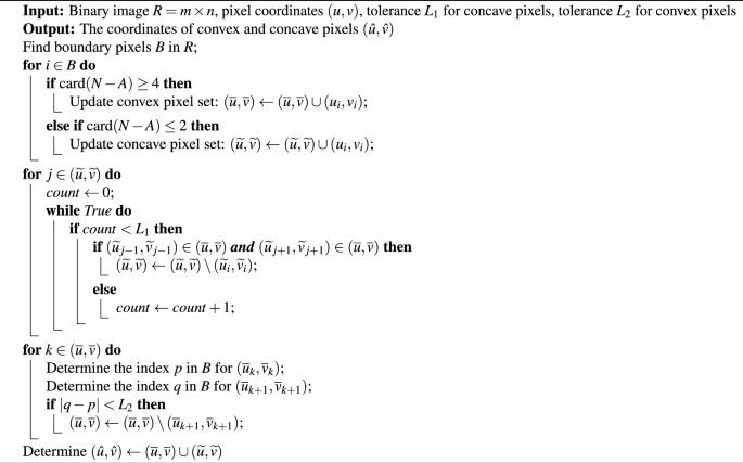
Convex and concave pixels extraction

Contour reconstruction and coordinate transformation

The contour can be reconstructed using B-spline after obtaining convex and concave pixels, with the reconstructed contour coordinates described by the pixel coordinate system (u-v). In order to enable the reconstructed contour to be used for subsequent analysis and calculation, (u-v) should be transformed into the world coordinate system (x-y). The coordinate transformation relationship is given by:

$$\begin{aligned} \begin{bmatrix} x^{*} \\ y^{*} \end{bmatrix} = \frac{1}{pps} \begin{bmatrix} u-u_{0} \\ v-v_{0} \end{bmatrix} + \begin{bmatrix} x_{0} \\ y_{0} \end{bmatrix} \end{aligned}$$

(5)

where coordinates (u, v) and $(x^{*},y^{*} )$ represent the pixel coordinates before transformation and the world coordinates after transformation of a certain point on the reconstructed contour, respectively; parameter pps denotes the number of pixels per unit dimension, which can be calculated through the relationship between the physical dimensions of the target contour and its pixel count in the image; $(u_{0},v_{0} )$ and $(x_{0},y_{0} )$ are reference points in the two coordinate systems, which can be set to the origin.

The presence of the parameter pps implies that the precision of the coordinate transformation in Eq. (5) is influenced by the image resolution. For a precise coordinate (x, y) on the target contour corresponding to a certain point coordinate $(x^{*},y^{*} )$ on the reconstructed contour, they should satisfy condition $\underset{R \rightarrow \infty }{lim}\left( x^{*},y^{*}\right) =\left( x,y \right)$. Hence, a high-resolution image is key to ensuring the precision of the reconstruction. It should be noted that, in this paper, the image resolution $R=m\times n$ is defined as the number of pixels contained within the smallest rectangular area encompassing the envelope curve.

Validation examples

Simulated examples

Simulated examples were used to quantitatively assess the accuracy of the proposed method and validate its effectiveness, as shown in Fig. 3. Reliable contour extraction typically requires a binary image; for simplicity, all subsequent analyzes were performed directly on binary images. The test image, shown in Fig. 3a, has a pixel resolution of $R=2880 \times 3000$ pixels. Both $L_1$ and $L_2$ were adopted as 2. Figure 3b shows some of the extracted convex and concave pixels and the contour reconstructed by cubic B-splines, which presents the accurate reconstruction results. In particular, almost all salient corners of the target configuration are composed of convex pixels, indicating that convex pixels carry the dominant shape information. The variation in the number of convex and concave pixels with respect to $L_1$ and $L_2$ is plotted in Fig. 3c. The increase in $L_2$ significantly suppresses the number of convex pixels, implying that an excessively large $L_2$ may lead to the loss of important contour details. In contrast, the number of concave pixels is small and is essentially insensitive to $L_1$. Reconstructions obtained with $L_2$ = 3 and $L_2$ = 4 (shown in Fig. 3(d)) already show a noticeable loss of detail, suggesting that $L_2$ should not exceed 3. Consequently, the recommended values for both $L_1$ and $L_2$ are 2 or 3. In the following discussions, $L_1$ and $L_2$ were adopted as 2.

The point with $(u_0,v_0)$=(0, 2351) pixels was selected as the reference and aligned with the world coordinate system, origin $(x_0,y_0)=(0,0)$. The pps can be the following:

$$\begin{aligned} pps=\frac{m}{x_{max}-x_{min}} \nonumber \\ \end{aligned}$$

(6)

where $x_{max}-x_{min}$ is the size of the target contour on the x axis of the world coordinate system, and $x_{max}-x_{min}=1000$ mm was adopted. The reconstructed contour is shown in Fig. 4.

To quantify the influence of image resolution on reconstruction accuracy, tests were conducted at four different resolutions, $R=2440 \times 2500, 1920 \times 2000, 1440 \times 1500$ and $960 \times 1000$ pixels (shown in Fig. 5). The contour extracted at the highest resolution ($R=2880 \times 3000$ pixels) was adopted as the standard value. As illustrated in Fig. 4, 130 points were sampled along this reference contour, starting from the reference point. For each corresponding point i on the lower-resolution contours, the vertical discrepancy was defined as $\Delta y=y_i-\overline{y}_i$, where $\overline{y}_i$ denotes the standard coordinate and $y_i$ is the coordinate obtained at the lower-resolution contour. The reconstruction error of the contour was evaluated using the root mean square error(RMSE):

$$\begin{aligned} RMSE=\sqrt{\frac{\sum _{i=1}^{n} (\Delta y)^2}{n} } \end{aligned}$$

(7)

The reconstruction errors are presented in Fig. 5b. The RMSE varies only between 0.477 mm and 0.641 mm, confirming that the accuracy of the proposed algorithm is essentially resolution independent within the adopted range of resolution and demonstrating its robustness. Although Table 1 shows that the number of control points changes significantly with resolution, this variation exerts a negligible influence on the reconstruction error. This observation indicates that the extracted control points effectively capture the salient pixel-level characteristics of the contour, so that moderate alterations in image resolution do not compromise the final result.

However, the reconstruction error originates predominantly from the inherent approximation error of the B-spline fitting and the uncertainty in pps. The magnitude of the latter is governed by the image resolution. Compared with the B-spline fitting error, controlling the image resolution is more effective in regulating the reconstruction error. Therefore, adjusting the image resolution serves as a primary approach for error control.

Fig. 3

Simulated example: (a) Contour with $R=2880\times 3000$ pixels, (b) reconstructed contour with convex (partially displayed) and concave pixels, (c) number of convex and concave pixels at different $L_1$ and $L_2$, and (d) comparison of contour anomalies at $L_2=3$ and $L_2=4$.

Fig. 4

The distribution of error evaluation points.

Fig. 5

Reconstructed errors at different image resolutions: (a) Contour at $R=2400\times 2500$, $1920\times 2000$, $1440\times 1500$, and $960\times 1000$ pixels, and (b) errors at evaluation points.

Table 1 Number of control points at different image resolutions.

The robustness of the proposed algorithm to image noise was further investigated. To isolate this effect from the variability of contour detection routines, zero-mean Gaussian noise was added directly to the coordinates of the control points. Figure 6 illustrates the resulting reconstructions for the image with $R=2880 \times 3000$ pixels. As the standard deviation $\sigma$ increases, the reconstruction error increases monotonically. The RMSE reaches 2.4 mm and the contour begins to deviate visibly at $\sigma$ = 10 pixels. When $\sigma$ = 20 pixels, the boundary oscillates significantly, yielding an RMSE of 4.6 mm. These results indicate that the proposed algorithm remains effective even under pronounced noise, highlighting its robustness. However, when the noise level becomes excessively high, the accuracy of the reconstructed contours is significantly compromised. To ensure precise reconstruction, the deviation in control point coordinates caused by image noise should preferably not exceed 10 pixels.

Fig. 6

Reconstruction results at different levels of the Gaussian noise: (a) Contours at $\sigma$=0.5, 10, and 20 pixels, and (b) RMSE from $\sigma =0.5$ to $\sigma =20$ pixels.

Real examples

Four industrial precision parts were used as reconstruction samples to verify the practical efficacy of the proposed method. The sample images and their binarized versions are shown in Fig. 7a and b, respectively, which belong to the complex connected domain. The internal and external boundaries can be separately extracted as control points and reconstructed, and then data fusion can be performed. The image resolutions for the four samples are $R=266 \times 284$, $392 \times 359$, $335 \times 356$, and $841 \times 443$ pixels, respectively. The reconstruction results, as shown in Fig. 7c, demonstrate results with high reconstruction accuracy and good smoothness.

Fig. 7

Reconstruction of the planar contour of industrial precision parts: (a) Original images, (b) binary images, and (c) reconstructed contour images.

Fig. 8

Reconstruction of the layout of the local traces in Micro-PCB: Located (a) in the bottom left corner and (b) in the right corner.

A Micro-PCB features intricate printed circuits, and the layout of its local traces can be extracted using the proposed algorithm. When extracting the contours, it is necessary to specify the computational objects of the algorithm, which are the numerous independent traces, and then sequentially reconstruct the distribution of traces in local areas. The extraction results are shown in Fig. 8a and b, demonstrating that the algorithm exhibits good applicability.

Conclusion

This paper presents a B-spline contour reconstruction algorithm based on the convexity and concavity of image contour, aiming to achieve a contour reconstruction method based on B-Spline that is both highly accurate and straightforward to implement. The optimal set of control points has been identified by employing convex and concave pixels as control points and leveraging the distribution characteristics of pixels within their eight-neighborhood, in conjunction with the application of constraints for filtering non-control points. The results of simulated and real examples demonstrate that the control points extracted using this method can reconstruct contour with high accuracy and good smoothness. In addition, the influence of image resolution and noise on the reconstruction was investigated in the simulated examples, demonstrating the strong robustness of the proposed algorithm.

References

Litjens, G. et al. A survey on deep learning in medical image analysis. Med. Image Anal. 42, 60–88. https://doi.org/10.1016/j.media.2017.07.005 (2017).
Raj, S. & Ray, K. C. Automated recognition of cardiac arrhythmias using sparse decomposition over composite dictionary. Comput. Methods Prog. Biomed. 165, 175–186. https://doi.org/10.1016/j.cmpb.2018.08.008 (2018).
Thompson, M. K. et al. Design for additive manufacturing: Trends, opportunities, considerations, and constraints. CIRP Ann. 65, 737–760. https://doi.org/10.1016/j.cirp.2016.05.004 (2016).
Kok, J. et al. Automatic generation of subject-specific finite element models of the spine from magnetic resonance images. Front. Bioeng. Biotechnol. 11, 35–44. https://doi.org/10.3389/fbioe.2023.1244291 (2023).
Kok, J. et al. Finite element mesh generation for composites with ply waviness based on x-ray computed tomography. Adv. Eng. Softw. 58, 35–44. https://doi.org/10.1016/j.advengsoft.2013.01.002 (2013).
Punarselvam, E. & Suresh, P. Investigation on human lumbar spine MRI image using finite element method and soft computing techniques. Clust. Comput. 22, 13591–13607. https://doi.org/10.1007/s10586-018-2019-0 (2019).
Liu, N.-Z., Zou, Y.-S., Ma, X.-F., Li, N. & Wu, S. Study of hydraulic fracture growth behavior in heterogeneous tight sandstone formations using CT scanning and acoustic emission monitoring. Pet. Sci. 16, 396–408. https://doi.org/10.1007/s12182-018-0290-6 (2019).
Zhao, Z., Zhao, Y., Jiang, Z., Guo, J. & Zhang, R. Investigation of fracture intersection behaviors in three-dimensional space based on CT scanning experiments. Rock Mech. Rock Eng. 54, 5703–5713. https://doi.org/10.1007/s00603-021-02587-9 (2021).
Shamshad, F. et al. Transformers in medical imaging: A survey. Med. Image Anal. 88, 102802. https://doi.org/10.1016/j.media.2023.102802 (2023).
Han, X.-F., Laga, H. & Bennamoun, M. Image-based 3d object reconstruction: State-of-the-art and trends in the deep learning era. IEEE Trans. Pattern Anal. Mach. Intell. 43, 1578–1604. https://doi.org/10.1109/TPAMI.2019.2954885 (2019).
Li, Y. Research and application of deep learning in image recognition. In booktitle2022 IEEE 2nd International Conference on Power, Electronics and Computer Applications (ICPECA), 994–999, https://doi.org/10.1109/ICPECA53709.2022.9718847 (2022).
Wu, W.-Y. & Wang, M.-J.J. Detecting the dominant points by the curvature-based polygonal approximation. CVGIP Gr. Models Image Process. 55, 79–88. https://doi.org/10.1006/cgip.1993.1006 (1993).
Chekol, B., Celebi, N. & TAŞCI, T. Segmented character recognition using curvature-based global image feature. Turkish J. Electr. Eng. Comput. Sci.,27, 3804–3814, https://doi.org/10.3906/elk-1806-195 (2019).
Kleppe, A. L., Tingelstad, L. & Egeland, O. Coarse alignment for model fitting of point clouds using a curvature-based descriptor. IEEE Trans. Autom. Sci. Eng. 16, 811–824. https://doi.org/10.1109/TASE.2018.2861618 (2018).
Ho, H. T. & Gibbins, D. Curvature-based approach for multi-scale feature extraction from 3D meshes and unstructured point clouds. IET Comput. Vis. 3, 201–212. https://doi.org/10.1049/iet-cvi.2009.0044 (2009).
Fernández-García, N. L., Martínez, L.D.-M., Carmona-Poyato, Á., Madrid-Cuevas, F. J. & Medina-Carnicer, R. Assessing polygonal approximations: A new measurement and a comparative study. Pattern Recognit. 138, 109396. https://doi.org/10.1016/j.patcog.2023.109396 (2023).
De Goes, F., Cohen-Steiner, D., Alliez, P. & Desbrun, M. An optimal transport approach to robust reconstruction and simplification of 2d shapes. In booktitleComputer Graphics Forum, Vol. 30, 1593–1602 (publisherWiley Online Library, addressOxford, UK, 2011).
García, N. L. F., Martínez, L.D.-M., Poyato, Á. C., Cuevas, F. J. M. & Carnicer, R. M. Unsupervised generation of polygonal approximations based on the convex hull. Pattern Recognit. Lett. 135, 138–145. https://doi.org/10.1016/j.patrec.2020.04.014 (2020).
Panagiotakis, C. Particle swarm optimization-based unconstrained polygonal fitting of 2d shapes. Algorithms 17, 25. https://doi.org/10.3390/a17010025 (2024).
Aguilera-Aguilera, E. J., Carmona-Poyato, A., Madrid-Cuevas, F. J. & Medina-Carnicer, R. The computation of polygonal approximations for 2d contours based on a concavity tree. J. Vis. Commun. Image Represent. 25, 1905–1917. https://doi.org/10.1016/j.jvcir.2014.09.012 (2014).
Jiang, H., Ben-chi, J., Lian, X. & Da-Zhu, L. A b-spline curve fitting algorithm based on contour key points. Appl. Math. Mech. 1000–0887(36), 423–31. https://doi.org/10.3879/j.issn.1000-0887.2015.04.010 (2015).
Bello, S. A., Yu, S., Wang, C., Adam, J. M. & Li, J. Deep learning on 3d point clouds. Remote Sens. 12, 1729. https://doi.org/10.3390/rs12111729 (2020).
Yang, Y., Fang, H., Fang, Y. & Shi, S. Three-dimensional point cloud data subtle feature extraction algorithm for laser scanning measurement of large-scale irregular surface in reverse engineering. Measurement 151, 107220. https://doi.org/10.1016/j.measurement.2019.107220 (2020).
Sa, J. et al. Depth grid-based local description for 3d point clouds. Signal, Image Video Process. 18, 4085–4102. https://doi.org/10.1007/s11760-024-03056-w (2024).
Shen, W., Wang, X., Wang, Y., Bai, X. & Zhang, Z. Deepedge: A multi-scale bifurcated deep network for top-down contour detection, https://doi.org/10.1109/CVPR.2015.7299067 (2015). notePaper presented at IEEE Conference on Computer Vision and Pattern Recognition, Boston Massachusetts, 15 October 2015.
Bertasius, G., Shi, J. & Torresani, L. Deepcontour: A deep convolutional feature learned by positive-sharing loss for contour detection, https://doi.org/10.1109/CVPR.2015.7299024 (2015). notePaper presented at IEEE Conference on Computer Vision and Pattern Recognition, Boston Massachusetts, 15 October 2015.
Guptha, N. S., Balamurugan, V., Megharaj, G., Sattar, K. N. A. & Rose, J. D. Cross lingual handwritten character recognition using long short term memory network with aid of elephant herding optimization algorithm. Pattern Recognit. Lett. 159, 16–22. https://doi.org/10.1016/j.patrec.2022.04.038 (2022).
Tong, Y. et al. Mathematical representation of 2d image boundary contour using fractional implicit polynomial. Optoelectron. Lett. 19, 252–256. https://doi.org/10.1007/s11801-023-2199-6 (2023).
Funding
This research work was supported by the National Key Research and Development Program of China NOs. 2023YFF0616800, the supports are gratefully acknowledged.
Author information
Authors and Affiliations
Contributions
B.W. is responsible for principle, analysis, investigation, and writing original draft preparation. Y.F.L., C.S., S.P.M., and J.B.C are responsebie for supervision, validations, writing-review and editing final manuscript. All authors discuss the results and contribute to the final manuscript.
Corresponding author
Ethics declarations
Competing interests
The authors declare no competing interests.
Additional information
Publisher’s note
Springer Nature remains neutral with regard to jurisdictional claims in published maps and institutional affiliations.
Rights and permissions
Open Access This article is licensed under a Creative Commons Attribution-NonCommercial-NoDerivatives 4.0 International License, which permits any non-commercial use, sharing, distribution and reproduction in any medium or format, as long as you give appropriate credit to the original author(s) and the source, provide a link to the Creative Commons licence, and indicate if you modified the licensed material. You do not have permission under this licence to share adapted material derived from this article or parts of it. The images or other third party material in this article are included in the article’s Creative Commons licence, unless indicated otherwise in a credit line to the material. If material is not included in the article’s Creative Commons licence and your intended use is not permitted by statutory regulation or exceeds the permitted use, you will need to obtain permission directly from the copyright holder. To view a copy of this licence, visit http://creativecommons.org/licenses/by-nc-nd/4.0/.
About this article
Cite this article
Wang, B., Li, Y., Sun, C. et al. B-spline contour reconstruction algorithm based on image contour concavity and convexity. Sci Rep 15, 41567 (2025). https://doi.org/10.1038/s41598-025-25414-5
Received:
Accepted:
Published:
Version of record:
DOI: https://doi.org/10.1038/s41598-025-25414-5