
Abstract
Accurate electricity demand forecasting is crucial for the stable operation of smart grids, as it enables proactive resource allocation and prevents grid failures caused by demand–supply mismatches. However, achieving precise predictions requires modeling both temporal consumption patterns and peak variations in electricity usage data. Regional power consumption data may contain sensitive commercial information, while federated learning (FL) offers a privacy-preserving approach to address data scarcity. Nevertheless, existing FL approaches struggle with two critical limitations: (1) the inherent risk of overfitting when modeling peak demand variations with sparse client-side data, and (2) the loss of client-specific features during the aggregation process, which can result in over-smoothing of predictions for some clients due to parameter inconsistencies across local models. To overcome these challenges, this paper proposes a Federated Two-Edge Graph Attention Network with Weighted Global Aggregation (FapDGN) for electricity demand forecasting. The FapDGN framework initiates by constructing a hybrid feature representation that simultaneously encapsulates both temporal dynamics and numerical fluctuations in electricity consumption patterns. Recognizing that temporal characteristics are crucial for prediction accuracy while peak variations pose higher overfitting risks, the system employs two-edge graph structures to process these elements independently. Specifically, it utilizes temporal edges in graphs coupled with a multi-scale attention mechanism to capture consumption trends over time, while implementing dynamic covariance through numerical structure edges in graphs to represent peak variations as parameterized Gaussian distributions, an approach that mitigates overfitting. The model subsequently combines these extracted temporal and peak variation features to produce its final predictive outputs. Furthermore, to combat potential over-smoothing issues, FapDGN integrates a similarity-based adaptive dynamic fusion mechanism for parameter aggregation at the server level when building the global model. Experimental results show that FapDGN outperforms commonly used FL methods in forecasting electricity demand.
Introduction
As smart grid technologies advance at an unprecedented pace, precise electricity consumption prediction has grown increasingly critical for effective power grid administration and control1,2. Numerous time-series based prediction approaches have been developed and adopted in current practice. Nevertheless, accurately capturing consumption peak dynamics remains particularly problematic in real-world applications. The implementation hurdles stem from both the fragmented nature of electricity usage data (distributed among various stakeholders like utility providers and manufacturing facilities) and the necessary confidentiality safeguards for proprietary industrial data. Such data fragmentation leads to informational silos that hinder consolidation, resulting in conventional forecasting models being constrained by inadequate training datasets and diminished accuracy. Federated learning presents itself as an optimal resolution to these challenges.
Federated learning (FL) represents a groundbreaking distributed machine learning framework that provides innovative solutions to data fragmentation challenges3,4,5. Nevertheless, existing FL-based electricity consumption forecasting approaches still exhibit certain limitations that require further investigation. When applied to electricity demand prediction, conventional FL techniques confront two primary obstacles that substantially affect prediction efficacy. The initial challenge pertains to mitigating overfitting in scenarios with constrained client datasets. In FL implementations, each participant possesses limited electricity usage records that may inadequately represent the full spectrum of consumption behaviors and peak fluctuations across various geographical areas or temporal periods. Overfitting becomes particularly concerning when prediction models become overly specialized to the restricted data patterns of individual clients, consequently impairing their adaptability to novel data instances. This issue is especially pronounced when modeling demand peak variations, given their inherently volatile and sporadic nature which renders them more susceptible to overfitting. The secondary challenge emerges during the model aggregation phase of FL, where locally trained models from multiple participants are consolidated into a unified global model. This aggregation process risks diminishing or erasing client-specific characteristics (such as distinctive consumption trends or regional peak behaviors), ultimately producing a global model that fails to adequately represent the heterogeneity of client data. This phenomenon, often referred to as over-smoothing, manifests as excessively generalized predictions that deviate from actual demand patterns for specific clients. Additionally, discrepancies in local model parameters stemming from variations in training data or model architectures can further amplify this problem.
To address the above issues, this paper proposes a Federated Two-Edge Graph Attention Network with Weighted Global Aggregation for Electricity Consumption Demand Forecasting (FapDGN). The FapDGN framework addresses key challenges in federated learning by developing a two-edge graph neural network architecture specifically designed for electricity load forecasting. This innovative approach operates within the FL paradigm to simultaneously tackle both overfitting and over-smoothing issues through its specialized design. The framework contains three core components: (1) A hybrid feature representation system that integrates sequence analysis techniques to comprehensively characterize electricity consumption data, effectively capturing both temporal dependencies and numerical fluctuations in demand patterns. (2) A two-edge graph neural network architecture that employs separate modeling pathways for distinct aspects of consumption data. The temporal pathway utilizes graph structures based on sequential relationships, while the numerical pathway focuses on correlations between consumption values. Within this architecture, the temporal pathway incorporates a multi-scale graph attention mechanism to extract consumption patterns across different time scales, whereas the numerical pathway applies dynamic covariance analysis to model peak variations as parameterized Gaussian distributions, with covariance volatility serving as a regularization mechanism to prevent overfitting. These two pathways synergistically combine their outputs to produce comprehensive predictions. (3) An advanced server-side aggregation protocol that introduces dynamic fusion mechanisms between local and global models. This protocol incorporates similarity-based weighting parameters during global model construction to preserve client-specific characteristics, thereby mitigating the over-smoothing phenomenon that typically occurs in conventional FL approaches. Experimental results demonstrate that the proposed method achieves better forecasting performance compared to traditional methods. The main contributions of this paper are as follows:
-
1.
The paper proposes a Federated Two-Edge Graph Attention Network with Weighted Global Aggregation (FapDGN) that separately models the temporal features and peak variation patterns of electricity consumption. By incorporating sequence analysis and graphs in 2 pathways, FapDGN mitigates overfitting caused by limited client-side data and accurately captures consumption fluctuations, particularly peak variations.
-
2.
The paper proposes a novel dynamic weighted fusion aggregation method at the server level, which incorporates similarity parameters during the global model construction to prevent over-smoothing. This method ensures that the global model retains client-specific features, leading to improved prediction accuracy and generalization across diverse consumption patterns.
The structure of this paper is organized as follows: Section "Related works" reviews related work on electricity consumption forecasting. In Section "Proposed model", we present the proposed FapDGN framework. Section "Experiments" provides experimental validation of the effectiveness of the proposed FapDGN, while the final section concludes the paper.
Related works
Traditional machine learning–based electricity consumption prediction methods
Conventional approaches for electricity demand forecasting primarily encompass three categories: temporal sequence analysis, statistical regression, and grey system theory6. Among these, autoregressive models like ARIMA process historical consumption data to project future trends, though they inherently rely on statistical stationarity assumptions and exhibit vulnerability to anomalous data points7. Regression techniques, including multivariate linear analysis, attempt to correlate consumption metrics with explanatory variables, yet struggle to capture intricate nonlinear dependencies between features8. Grey prediction models demonstrate particular utility in data-scarce scenarios, though their effectiveness diminishes considerably when extending forecast horizons beyond short-term projections9.
Deep learning–based electricity consumption prediction methods
The evolution of machine learning has brought about a revolutionary change in electricity consumption forecasting. Advanced techniques exhibit varying degrees of efficacy across diverse scenarios. Among them, neural network architectures have emerged as highly potent tools. Deep learning models are proficient in automated feature extraction and the recognition of complex nonlinear patterns. Notably, specialized recurrent neural networks such as Long Short—Term Memory (LSTM) have manifested exceptional performance in temporal sequence modeling, attaining state—of—the—art outcomes in load forecasting applications.
Nevertheless, these data—intensive approaches generally necessitate substantial centralized datasets to achieve optimal training performance. This requirement becomes a challenge when faced with the data fragmentation issues inherent in distributed energy systems. The development of deep learning methodologies has introduced several innovative paradigms in this field. Early breakthroughs laid the foundation for temporal modeling. Subsequently, advancements like multi—scale LSTM implementations enhanced pattern recognition capabilities through hierarchical feature extraction. Bidirectional variants of these models further improved predictive accuracy by integrating contextual information from both temporal directions. More recently, hybrid architectures have gained prominence. They combine recurrent networks with probabilistic modeling techniques and ensemble strategies that integrate unsupervised learning with traditional feature selection methods. Complementary to these approaches, frequency—domain analysis techniques have developed in parallel, offering alternative perspectives through signal decomposition methods and spectral analysis. While Fourier—based neural networks can effectively capture periodic patterns, they often face limitations in balancing temporal precision and frequency resolution, potentially neglecting transient characteristics. Wavelet transform—based solutions address this problem by adopting adaptive decomposition techniques tailored to the heterogeneous nature of energy consumption data.
Federated learning applications
The distributed learning paradigm has exhibited its adaptability across diverse domains. Specifically, in the healthcare sector, it promotes collaborative model development among medical institutions for disease diagnosis while ensuring patient confidentiality10. In the financial domain, it enables banks to jointly improve fraud detection capabilities while protecting sensitive transaction data11. These applications highlight the paradigm’s efficacy in resolving data fragmentation issues. However, its application in load forecasting remains relatively under—investigated, with only a limited amount of research focusing on model refinement and performance improvement. The standard operational framework of such algorithms, as exemplified by FedAvg1, involves iterative processes of client—side training, parameter aggregation, and global model dissemination. This process faces significant challenges when dealing with data heterogeneity, which is characterized by non—identical client data distributions, mainly manifested through label distribution skew and domain shift. To address these challenges, current methods can be generally divided into two optimization categories: enhancement of client training and refinement of the aggregation mechanism. Client—side optimization techniques include gradient adjustment methods that use control variables to quantify and correct update disparities, model comparison approaches that apply similarity constraints to prevent local overfitting, and loss function augmentation techniques that incorporate regularization terms to restrict parameter divergence from the global model.
Proposed model
This paper proposes Federated Two-Edge Graph Attention Network with Weighted Global Aggregation (FapDGN) for electricity consumption demand forecasting. The model structure of FapDGN is shown in the Fig. 1.

The structure of the proposed FapDGN.
Next, the paper details the model specifics.
Problem formulation and setup
This research employs a distributed machine learning framework where K independent participants jointly develop a predictive model without disclosing their proprietary datasets (D = {D1, D2,…, DK}). Each participant processes its own historical consumption sequence (x) to generate localized demand forecasts. The collaborative training process seeks to establish a unified predictive model capable of accurately anticipating electricity usage patterns across all participants, thereby achieving the core objective of federated load forecasting.
where, Li is the loss of i-th local model, \(\gamma_{i}\) is the weight of the i-th local model. This paper proposes an electricity consumption demand forecasting method based on FapDGN. The specific process is as follows:
Electricity consumption demand forecasting model construction
Electricity consumption data inherently possesses the 2 attributes: the temporal dimension reflects the variation in electricity consumption over time, with consumption changing along the time series. The spatial dimension reflects the numerical correlation between the peak fluctuations in electricity consumption data. The prediction of current electricity consumption data relies on the trend of temporal changes and the numerical correlation of consumption peak variations. Therefore, to model these attributes of electricity data, this paper designs Two-Edge Graphs.
Data preprocessing and two-edge graph construction
During the preprocessing stage, the original electricity consumption sequence is processed via moving abnormal noise in the data. Simultaneously, feature fusion enhancement is implemented. STL decomposition is employed online to partition the data into three components: [Trend Component T, Seasonal Component S, Residual Component R]. Subsequently, EEMD decomposition is applied to the electricity consumption data to acquire the IMF components. Consequently, for each time slice, the data vector f comprises [data, T, S, R, IMF1, …, IMFk], thereby constructing the representation of the electricity consumption data. Next, the Two-Edge Graphs for electricity consumption data are constructed. We represent electricity consumption data as a Two-Edge Graph:
The nodes of this Two-Edge Graphs are defined as follows:
Let the electricity consumption series be X = {× 1, × 2, …, xn} ∈ Rn∗d , where each time point xt corresponds to a graph node vt , and the node feature vector is ft = [xt , Tt , St , Rt, IMF1t,…, IMFkt ]. The TEGraph includes two types of edges. One type of edge is used to model the temporal relationships, represented as Edgetemp, with the corresponding adjacency matrix Atemp. The other type of edge models the numerical correlations in the electricity data, represented as Edgenum, with the corresponding adjacency matrix Anum. Specifically, the edge calculation process is as follows:
To model the temporal nature of electricity data, the temporal edges are defined as:
where, K represents the time window. In this scenario, nodes within the time series that are temporally nearer to the current time t will be assigned higher weights, and the weights of the connections will decay as time progresses. Until the distance from the current node t exceeds the window length, the connection weights will be set to 0. This aligns with the correlation pattern of electricity consumption that varies over time.
To ensure accuracy in the predicted values while modeling the temporal patterns of electricity consumption, we need to model the numerical correlations during the electricity consumption process. Based on these correlations, we guide the prediction of electricity demand for the current time slice. Therefore, we define the feature similarity edges Edgenum as follows:
Herein, τ represents the pre-defined numerical threshold. In this research, the value of τ is empirically determined by computing the average cosine similarity of all feature points within the dataset and designating it as τ. To preclude interference from excessively smooth and readily predictable electricity data, a threshold τ is established to filter out data exhibiting obvious volatility. Subsequently, based on the correlation of this data, the numerical relationships in the electricity consumption process are modeled.
Thus, we construct the Two-Edge Graphs. Next, we design a prediction model based on Graph Attention Neural Networks using these Two-Edge Graphs.
Graph attention neural network for electricity consumption demand forecasting
FapDGN designs an integrated graph attention mechanism to model the two-edge graphs
-
(1)
For temporal edges in graphsA multi-scale graph self-attention neural network is devised to extract attention features at diverse scales, while modeling temporal features with different time series lengths. Specifically, FapDGN utilizes a multi-scale graph attention network to extract multi-scale attention features, which encompasses three core components: (1) a similarity metric that quantifies the associations among nodes in the graph; (2) attention coefficients that reflect the differential influences of input relationships; and (3) aggregated attention features across multiple scales. The similarity between two input vectors is computed according to formula (5):
$$Similarity_{{_{ij} }}^{h} = {\text{SLP}}\left( {A_{temp}^{h} \times W^{h} \times f_{i} , \, A_{temp}^{h} \times W^{h} \times f_{j} } \right),$$(5)Here, Atemph represents the h-scale neighborhood of the graph adjacency matrix, Similarityijh denotes the h-scale similarity feature between nodes i and j, and Wh stands for the learnable weight matrix. Based on this h-scale similarity function, the h-scale attention coefficient is defined as shown in Eq. (6).
$$\alpha_{{_{ij} }}^{h} = {\text{softmax}} \left( {Similarity_{{_{ij} }}^{h} } \right),$$(6)Here, αijh is the attention coefficient. The FapDGN computes attention coefficients across H scales, and then derives the attention feature of node i based on these H-scale attention coefficients, as defined in Eq. (7).
$$feature_{i} = \, \sum\nolimits_{h}^{H} {\sum\nolimits_{j} {\alpha_{{_{ij} }}^{h} \times {\text{Q}}^{h} \times f_{j} } } ,$$(7)where, Qh is the learnable weightes.
-
2.
For numerical correlation edges in graphs
FapDGN designs a graph Gaussian autoencoder based on multi-hop attention to model the numerical features of electricity consumption. The multi-hop attention-based encoder designed in this paper is divided into 2 hops, filtering out the features most closely related to the current electricity consumption value.
First Hop Numerical correlation information filtering
Taking the attention features of node i as an example, the graph nodes of the input numerically correlated graph are first globally scanned to calculate the preliminary attention weights, and then significant regions or nodes are selected.
Second Hop Dependency relationship modeling
Based on the results of the first hop, the substructures within the selected regions are further analyzed.
Here, R is a learnable mask matrix that is randomly initialized. The 2-hop results are aggregated through a gating mechanism to form the final attention distribution.
Here, W1 and W2 are learnable parameters, and the features are parameterized as the mean and covariance of a Gaussian distribution. The decoder subsequently reconstructs attention-enhanced representations by synthesizing these weighted associations. Here, we encode features as parameterized Gaussian distributions, where W1 parameterizes the mean (expectation) of the Gaussian distribution and W2 parameterizes its covariance matrix. The volatility in electricity consumption data contains noise, and fully fitting the fluctuating data would lead to overfitting the noise. By using Gaussian distribution fitting, we mitigate noise overfitting through covariance fluctuation, the formula can be expressed as mean + disturbance variable × parameterized covariance matrix, where the disturbance variable follows a standard normal distribution. Thus, by sampling random disturbance values, controlled perturbations are introduced into the covariance term, alleviating noise overfitting. This process resembles the principle of dropout.
Electricity consumption forecasting based on all components
After the above steps, the final forecasting for the electricity consumption data is calculated by synthetizing the forecasted IMF components, as shown in Formula (11).
Here, SLP is a fully connected output layer that outputs the prediction result. The goal of the task is to minimize the following loss:
Here, CrossEntropy denotes the cross-entropy loss, λ represents the similarity metric coefficient used to balance the reconstruction loss and the cross-entropy, and we set it to 0.005 in this work.
Adaptive dynamic fusion parameter aggregation based on model parameter similarity
To address the over-smoothing problem of client—side models in the process of global model aggregation, this paper presents an adaptive parameter aggregation approach based on model parameter similarity. To solve this issue, an adaptive parameter aggregation method relying on dynamic weight assignment is devised. On the server side, the over-smoothing problem is alleviated through parameter difference detection and weight modification. Simultaneously, a global regularization term is introduced on the client side to prevent local models from overfitting to inconsistent model parameters.
-
1)
On the server side
Calculate the L2 distance Simi = Cosine(wi – wg) between the i − th local model parameter wi and the current global parameter wg. Here, we only use the parameters of the network model’s prediction layer, specifically those in Eq. (11), to compute similarity, thereby reducing computational complexity. Then, use the softmax function to compute the aggregation weight:
$$\alpha_{i} = {\text{softmax}} \left( {sim_{i} } \right)$$(13)Then, the new global model is aggregated following Formula (14):
$$Parameter_{g\_new} = \sum\nolimits_{i} {\alpha_{i} \times Parameter_{i} }$$(14) -
2)
On the client side
When updating the local model with the received global model, a global model regularization term is introduced, modifying the loss function as follows:
$$Loss = \frac{1}{N}\sum\nolimits_{n} {\left\{ \begin{gathered} \lambda \sum\nolimits_{i,j} {\left[ {\cos ine\left( {Z_{{_{i} }}^{n} , \, Z_{{_{j} }}^{n} } \right) - A_{num\_i,j} } \right]_{n}^{2} } + \hfill \\ \, CrossEntropy\left( {y^{n} , \, label^{n} } \right) \hfill \\ \end{gathered} \right\}} + \beta \left\| {Paremeter_{local} ,Paremeter_{global} } \right\|^{2}$$(15)where λ and β are hyperparameters, λ = 0.01 and β = 0.005 in the experiments.
Analysis of computational cost
The proposed FapDGN model consists of three components: (1) preprocessing of electricity consumption data, (2) the designed Two-Edge graph and its corresponding feature analysis network, and (3) aggregation of the global model. While the model introduces some additional operations, its complexity remains controllable. Specifically, in the preprocessing stage, STL decomposition and EEMD methods are primarily employed to extract signal features. The computational complexity of this stage can be expressed as Opre(l), where l represents the window size of the electricity consumption sequence. The second component involves the construction of the Two-Edge graph. Compared to traditional graph neural networks, this part introduces two additional network models, resulting in extra computational complexity dependent on the GNN used. In this paper, a 3-layer graph attention network is adopted, whose complexity is relatively controllable. The computational complexity of this stage can be expressed as Ognn(h), where h denotes the number of network layers. Finally, in the global aggregation stage, additional weighted calculations are introduced to measure the similarity between the parameters of each client model’s classification layer and those of the global model. The computational complexity of this stage is expressed as Osim(n), where n represents the number of nodes in the classification layer.
Therefore, the additional computational complexity of the proposed FapDGN can be summarized as: Opre(l) + Ognn(h) + Osim(n).
Experiments
In the experimental section, we validate the effectiveness of the proposed FapDGN. Our experiments conduct comparative analyses to assess three crucial conclusions: (1) the proposed FapDGN demonstrates superior performance compared to benchmarks in prediction tasks, (2) the proposed Two-Edge graphs exhibit advantages over traditional modeling approaches for electricity consumption data, and (3) the similarity-based adaptive parameter aggregation effectively mitigates parameter inconsistency during the global aggregation process. Among these, the first conclusion is validated in Section "Validating the effectiveness of FapDGN", while the second and third conclusions are verified in Section "Ablation experiments for FapDGN".
Next, we first introduce the datasets and experimental settings used in this paper in Section "DataSets and experiment settings". Then, in Section "Data availability statement", we describe the data sources, and in Section "Baselines for comparison", we present the baseline methods adopted for comparison. Section "Validating the effectiveness of FapDGN" contains the comparative experiments, and Section "Ablation experiments for FapDGN" presents the ablation studies.
DataSets and experiment settings
Introduction to datasets
This paper employs the experiments using 2 datasets.
-
(1)
The electricity consumption dataset, originally from Tetouan, Morocco (Electric Power Consumption on Data_kaggle)12, includes 52,416 observations recorded at 10-min intervals, each with 9 features: Date Time (timestamp per interval), Temperature (ambient weather), Humidity ( atmospheric moisture), Wind Speed ( wind velocity), General Diffuse Flows (low-temperature fluid discharge through geological and biological formations), Diffuse Flows, and Zone 1/2/3 Power Consumption (energy usage per zone). Environmental attributes: Temperature, Humidity, Wind Speed, and Diffuse Flows are incorporated as supplementary features in the vector f, though holiday data is absent. Figure 2 visualizes Zone 1’s consumption trends over a period of time.
Fig. 2 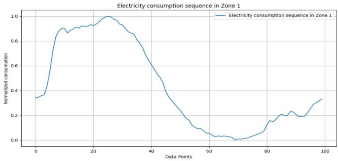
Electricity consumption data in Zone 1.
-
(2)
The second dataset on electricity consumption is derived from five regions within the operational area of China Southern Power Grid, covering five administrative divisions from December 1 2024 to May 31, 2025 (Data_Southern). This dataset includes hourly electricity consumption records for each region, with variations in user composition—such as industries, residential areas, and other sectors—across the different regions. These differences contribute to unique patterns in electricity consumption distribution. Figure 2 illustrates the electricity consumption data for a specific region within China Southern Power Grid over time.
As shown in Fig. 3, the electricity consumption data exhibits approximate periodicity and peak variations. These 2 datasets can be used for electricity prediction tasks.
Fig. 3 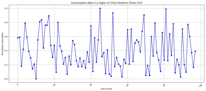
The consumption data in an area of the China Southern Power Grid.


Experiment settings
In experiments, the first dataset contains electricity consumption data from 3 different regions, while the second dataset contains electricity consumption data from 5 different regions. We use these electricity consumption data as data in different clients to create a federated learning environment to validate the effectiveness of the algorithm proposed FapDGN in this paper. When validating the effectiveness of the algorithm using these two datasets, we followed conventional procedures for dataset partitioning and preprocessing. Specifically, we first preprocessed the data by normalizing it to the range [0, 1] for computational convenience. We then removed abnormal noise from the data. The feature vectors used in the computation were [data, T, S, R, IMF1, …, IMFk]. Next, we split the data into training and testing sets, selecting 20% of the data as the test set. The selection method involved partitioning the data using a time-window approach, where the most recent 20% of the data was taken as the test set.
Baselines for comparison
This paper employs a set of benchmark models within the federated learning (FL) framework, comprising nine comparative algorithms categorized into three distinct groups to evaluate and compare their performance.
-
(1)
The first group integrates conventional electricity with representative federated learning frameworks such as AvgFL and FedCor, resulting in models including AvgFL-SVR, AvgFL-BiLSTM, AvgFL-Multi-Scale Attention (AvgFL-MSattention), FedCor-SVR, FedCor-BiLSTM, and FedCor-Multi-Scale Attention (FedCor-MSattention). Among these, SVR denotes the Support Vector Regression model, BiLSTM refers to the Bidirectional Long Short-Term Memory model, and the Multi-Scale Attention model captures hierarchical temporal dependencies. The Adaptive Stacked LSTM13 framework is also incorporated, which leverages adaptive learning, federated learning, and edge computing concepts for energy consumption
-
(2)
The second group of comparative algorithms employs data augmentation techniques to mitigate data heterogeneity and imbalance across clients. In this study, we adopt Fed CNN-LSTM14. In Fed CNN-LSTM, electricity consumption data is synthesized using Generative Adversarial Networks (GANs) to address client overfitting issues through data augmentation.
-
(3)
The third group leverages pretrained models to enhance the adaptability of prediction frameworks. Specifically, we employ SparseMoE15, where the expert network of the Mixture of Experts (MoE) architecture is implemented using a transformer-based deep learning model called Metaformer. This model utilizes Exponential Moving Average (EMA) operations and pooling mechanisms for prediction.
Validating the effectiveness of FapDGN
In the experimental section, we primarily validate the effectiveness of the proposed FapDGN model compared with nine benchmark models in terms of Mean Squared Error (MSE), Mean Absolute Error (MAE), and the fit degree of electricity consumption. The analysis is conducted separately using two datasets: Data_kaggle and Data_Southern.
Validating on Data_kaggle
For electricity consumption prediction, we verify the effectiveness of FapDGN using the Tetouan-Electricity-Consumption data (Data_kaggle). Tables 1 and 2 record the prediction results, showing the electricity consumption forecasts.
The experimental results summarized in Tables 1 and 2 for the Tetouan Electricity Consumption dataset clearly show that the proposed FapDGN model achieves the lowest MSE and MAE across all regions. Compared with conventional federated learning frameworks such as FedCor and AvgFL, as well as data-augmented approaches like Fed CNN-LSTM and adaptive methods such as Adaptive Stacked LSTM, FapDGN consistently delivers superior predictive accuracy. Notably, the model maintains strong robustness during periods of sharp demand fluctuations, indicating its enhanced capability to capture both baseline consumption patterns and sudden demand spikes. A visual comparison of the predicted and actual electricity consumption for Zone 1 is provided in Fig. 4.

The forecasted electricity consumption curve in Zone 1.
As shown in Fig. 4, the FapDGN model proposed in this paper has a higher degree of fitting compared to existing methods. Among the comparative algorithms, SparseMoE exhibits stronger fitting capability for electricity consumption data.
Validating on Data_Southern
In the subsequent experiments, we verify the forecasting performance of the FapDGN on the electricity consumption data within the China Southern Power Grid dataset. Tables 3 and 4 presents the forecasting performance of the FapDGN when utilizing the electricity consumption data from the China Southern Power Grid dataset. The results presented in Tables 3 and 4, in terms of the MSE and the test MAE.
As evidenced in Tables 3 and 4, FapDGN achieves the lowest MSE and MAE across all zones. This performance under-scores FapDGN’s enhanced capability in data fitting and predictive accuracy compared to conventional electricity consumption forecasting frameworks. The forecasted electricity consumption and the original electricity consumption in Zone 1 of Data_Sourthern are shown in Fig. 5.

The forecasted electricity consumption curve in Area 1 of Data_Sourthern.
As shown in Fig. 5, the FapDGN model proposed in this paper demonstrates a higher degree of fitting compared to existing methods, particularly in regions with electricity consumption fluctuations. Among the comparative algorithms, SparseMoE exhibits stronger fitting capability for electricity consumption data.
Ablation experiments for FapDGN
To verify the effectiveness of the proposed FapDGN framework, ablation studies are carried out on its core components: the Two- Edge graph, the Gaussian Graph Attention Autoencoder for modeling peak variations, and the dynamic fusion aggregation method. Four ablated variants are evaluated: 1) FapDGN-temp (eliminating the numerical structure edges in the Two-edge graph); 2) FapDGN-AE (replacing the Gaussian Graph Attention Autoencoder with an AE); 3) FapDGN-Avg (substituting the dynamic fusion aggregation method with the standard AvgFL); and 4) FapDGN-Att (replacing hierarchical encoding with conventional attention mechanisms). These variants are compared with the full FapDGN model on two real-world datasets for electricity consumption forecasting. The experimental results are presented as follows.
The ablation study results verify the effectiveness of the core components in the FapDGN framework. As shown in Tables 5 and 6, the full FapDGN model consistently outperforms its ablated variants across all zones in both datasets, achieving the lowest MSE values. This confirms that each component contributes significantly to the model’s performance. The FapDGN-Att variant, which replaces hierarchical encoding with conventional attention mechanisms, shows slightly higher MSE compared to the full model. This suggests that the hierarchical encoding in FapDGN better captures the complex patterns in electricity consumption data. Similarly, the FapDGN-AvgFL variant, which uses standard AvgFL instead of the dynamic fusion aggregation method, exhibits inferior performance, indicating that the dynamic fusion method more effectively integrates client models. The FapDGN-AE variant, replacing the Gaussian Graph Attention Autoencoder with a standard AE, shows marginally higher MSE, highlighting the importance of the Gaussian Graph Attention mechanism in modeling peak variations. The FapDGN-temp variant, which eliminates numerical structure edges, performs worse than the full model, demonstrating the necessity of the Two-Edge graph structure for capturing both temporal and numerical relationships in electricity data. The ablation study validates the effectiveness of each component in the FapDGN framework, with the full model achieving the best performance by leveraging its specialized design for electricity consumption forecasting.
Conclusion
This study introduces the Federated Two-Edge Graph Attention Network with Weighted Global Aggregation (FapDGN), a framework crafted to surmount significant limitations inherent in federated learning-based electricity consumption forecasting methodologies. By integrating a sophisticated hybrid feature representation strategy, a uniquely designed two-edge graph neural architecture, and advanced dynamic aggregation mechanisms, FapDGN adeptly tackles the twin issues of overfitting and over-smoothing that frequently undermine the efficacy of traditional approaches. The framework’s innovative capability to intricately model temporal dependencies, accurately capture numerical fluctuations, and discern client-specific patterns through its graph attention mechanisms and covariance regularization techniques, showcases an unparalleled level of prediction accuracy. This is particularly evident in its adept handling of demand peak dynamics. Rigorous experimental validation has unequivocally demonstrated the framework’s robustness in effectively managing fragmented industrial data, all while meticulously preserving data confidentiality. Looking ahead, future research endeavors delve into the real-time deployment of FapDGN within multi-stakeholder smart grid environments. In such contexts, the framework’s adaptive aggregation capabilities hold the potential to bolster grid stability and optimize energy management practices, thereby contributing to more efficient and resilient energy systems.
Data availability
This paper uses 2 datasets. The first electricity consumption dataset is obtained from Tetouan in Morocco and is available on (https://www.kaggle.com/datasets/fedesoriano/electric-power-consumption). The second dataset is available on (https://pan.baidu.com/s/1b3S-EBYeaiIcNwHGBUtSYw?pwd=ggtv).
References
Yildiz, B., Bilbao, J. I. & Sproul, A. B, A review and analysis of regression and machine learning models on commercial building electricity load forecasting. Renew. Sustain. Energy Rev. 73, 1104–1122 (2017).
González, A. M., Roque, A. S. & García-González, J. Modeling and forecasting electricity prices with input/output hidden Markov models. IEEE Trans. Power Syst. 20(1), 13–24 (2005).
Gomez, W., Wang, F. K. & Amogne, Z. E. Electricity load and price forecasting using a hybrid method based bidirectional long short-term memory with attention mechanism model. Int. J. Energy Res. 1, 3815063 (2023).
Zhang, X., Grolinger, K., Capretz, M. et al. Forecasting residential energy consumption: Single household perspective. In 17th IEEE International Conference on Machine Learning and Applications (IEEE, 2019).
Imani, M. Electrical load-temperature CNN for residential load forecasting. Energy 227, 120480 (2021).
Wang, S. et al. Bi-directional long short-term memory method based on attention mechanism and rolling update for short-term load forecasting. Int. J. Electrical Power Energy Syst. 109, 470–479 (2019).
Torres, J. F., Martínez-Álvarez, F. & Troncoso, A. A deep LSTM network for the Spanish electricity consumption demand forecasting. Neural .Comput. Appl. 34(13), 10533–10545 (2022).
Kim, N., Choi, J. LSTM based short-term electricity consumption forecast with daily load profile sequences. In IEEE 7th Global Conference on Consumer Electronics (IEEE, 2018).
Zheng, J., Xu, C., Zhang, Z et al. Electric load forecasting in smart grids using long-short-term-memory based recurrent neu-ral network. In 51st Annual Conference on Information Sciences and Systems (CISS). (IEEE, 2017).
Dedinec, A. et al. Deep belief network based electricity load forecasting: An analysis of Macedonian case. Energy 115, 1688–1700 (2016).
Tsai, C. L., Chen, W. T. & Chang, C. S. Polynomial-Fourier series model for analyzing and predicting electricity consumption in buildings. Energy Build. 127, 301–312 (2016).
https://www.kaggle.com/datasets/fedesoriano/electric-power-consumption.
Abdulla, N., Demirci, M. & Ozdemir, S. Smart meter-based energy consumption forecasting for smart cities using adaptive feder-ated learning. Sustain. Energy Grids Netw. 38, 101342 (2024).
De Moraes, S. E. M. et al. Forecasting energy power consumption using federated learning in edge computing device. Internet Things 25, 101050 (2024).
Wang, R. et al. Personalized federated learning for buildings energy consumption forecasting. Energy Build. 323, 114762 (2024).
Funding
This work was supported by the Science and Technology Project of China Southern Power Grid Co. Ltd (035900KK52222003).
Author information
Authors and Affiliations
Contributions
The concept and methodology of this paper were designed by Lukun Zeng, while the experiments and analysis were carried out by Ming Yang, Jianyu Ren, Sheng Li , and Yuan Ai. The writing of the paper was done by Lukun Zeng and Kaihong Zheng. The data organization and visualization were completed by Xiaohua Yang, Jianyu Ren, and Sheng Li. In addition, Kaihong Zheng’s other contributions include revising the paper based on the draft completed by Lukun Zeng and leading the revisions of this article. All authors reviewed the manuscript.
Corresponding author
Additional information
Publisher’s note
Springer Nature remains neutral with regard to jurisdictional claims in published maps and institutional affiliations.
Rights and permissions
Open Access This article is licensed under a Creative Commons Attribution-NonCommercial-NoDerivatives 4.0 International License, which permits any non-commercial use, sharing, distribution and reproduction in any medium or format, as long as you give appropriate credit to the original author(s) and the source, provide a link to the Creative Commons licence, and indicate if you modified the licensed material. You do not have permission under this licence to share adapted material derived from this article or parts of it. The images or other third party material in this article are included in the article’s Creative Commons licence, unless indicated otherwise in a credit line to the material. If material is not included in the article’s Creative Commons licence and your intended use is not permitted by statutory regulation or exceeds the permitted use, you will need to obtain permission directly from the copyright holder. To view a copy of this licence, visit http://creativecommons.org/licenses/by-nc-nd/4.0/.
About this article

Cite this article
Yang, M., Ren, J., Zeng, L. et al. Federated two-edge graph attention network with weighted global aggregation for electricity consumption demand forecasting. Sci Rep 15, 45792 (2025). https://doi.org/10.1038/s41598-025-28610-5
Received:
Accepted:
Published:
Version of record:
DOI: https://doi.org/10.1038/s41598-025-28610-5
