Identifying influential spreaders based on improving communication transmission model and network structure

Abstract

The identification of key nodes has garnered considerable attention across various research domains, including commercial marketing, infectious disease prevention and control, road network optimization, intelligent electricity management, and Chinese medicine formulation design. To evaluate critical nodes within complex networks, numerous algorithms have been proposed. However, these methods exhibit certain limitations such as one-sided considerations and single evaluation indexes. Consequently, the applicability of these key node identification approaches is limited to specific scenarios. In this paper, we propose a novel method for identifying key nodes based on principles from communication transmission theory and the law of gravity. Our approach fully explores the network structure and node relationships, integrating the Shannon channel capacity model and the gravity model. This method not only considers a node’s own location and importance, but also the proximity of its neighbors to the target node within two hops. Through extensive experimentation, we demonstrate that our algorithm outperforms representative methods proposed in recent years in terms of consistency with the SIR model, similarity of Top-N nodes, and node importance differentiation. Real-world experiments conducted on COVID-19 networks further validate the effectiveness of our approach.

Introduction

In reality, many networks can be abstracted as complex networks, including disease propagation networks¹, social networks², biological networks³, rumor⁴ and information dissemination networks⁵. Accurately identifying the important nodes within networks is crucial for studying network properties and predicting propagation, given that the influence of nodes in these networks is not consistent.

Current research on key nodes is mainly divided into two categories. The first category involves quantifying the value of each node in the network and ranks all nodes, with the top-ranked nodes indicating a higher influence in the network. The second category aims to find the smallest set of nodes critical to the network’s structure or function, such as selecting the optimal seed node set in social networks⁶ or identifying the lowest-cost check-in nodes⁷. This paper mainly focuses on the research within the first category.

Several key node identification methods have been proposed, including basic algorithms such as degree centrality (DC)⁸, k-shell⁹, betweenness centrality¹⁰, clustering coefficient¹¹, eigenvector centrality (EC)¹², and PageRank¹³. While these models uncover certain important characteristics of nodes, they often consider only a single factor. However, real-world networks exhibit a high degree of intricacy in their interdependencies among elements within and across networks. To address this issue, researchers have endeavored to enhance existing algorithms by integrating additional factors such as clustering coefficient¹⁴, network hierarchy¹⁵, neighbor conditions¹⁶, and distances^17,18 to identify nodes that maximize influence. Several approaches exist for quantifying the information entropy¹⁹ and collective influence²⁰ of nodes within networks. Some studies have explored the use of Laplacian energy^21,22 based on node degree or improved the k-shell and closeness centrality models to optimize node evaluation²³. Comprehensive models incorporating multiple underlying algorithms have been devised to provide a more thorough assessment of a node’s influence^24,25,26. However, these models have the disadvantage of not maximizing the positive aspects of a specific underlying algorithm.

Consequently, the integration of a suitable mathematical model provides a reliable mechanism to precisely assess the capabilities of individual nodes. Scholars have conducted extensive research on complex networks in recent years, notably leveraging the classical gravity model initially proposed by Ma²⁷. However, the model exclusively considers the spatial positioning and proximity of the target node and its neighboring nodes. Li et al.²⁸ made improvements by incorporating degree as mass and replacing the distance with the truncated radius, which reduced computational complexity to some extent. Nevertheless, fewer factors were still considered. Zhong et al.²⁹ designed the coefficients and masses based on the gravity model, ensuring that the importance of nodes is not solely determined by their degree and k-shell values but also influenced by the propagation rate. To address this issue, several studies^{30,31,32,33,34} have enhanced the gravity model by incorporating a combination of node shell values, degree values, eigenvectors, clustering coefficients, and other fundamental parameters. Experimental findings from related studies suggest that the incorporation of the gravity model improves the identification of important nodes. However, due to the intricate and dynamic relationships among network elements, solely relying on a single mathematical model in complex networks hinders further enhancement of node identification effectiveness. Thus, this paper conducts an in-depth investigation into the existing issues while considering these factors.

Sun et al. analyzed the characteristics of social circles in real society and introduced the Matthew effect from psychology into the study of complex networks³⁵. Similarly, to better align the proposed node identification method with real-world scenarios, this study undertakes a comprehensive analysis of social networks in section "Basic idea", considering their distinctive characteristics. Subsequently, the algorithm’s core concept is introduced.

Basic idea

The study of nodal importance revolves around identifying individuals with higher influence within a network. To illustrate the core concept, a small social network comprising 13 individuals (nodes) connected by 19 edges was constructed, as depicted in Fig. 1. The study delves into the following aspects:

• (1) Direct neighbor influence. The strength of a node’s influence within the network correlates with the cumulative sum of the k-shell values of its one-hop neighboring nodes and the sum of the degree values of its nearest neighbors. A higher value in these metrics indicates that the node possesses a greater number of significant neighbors, thereby amplifying its impact on the overall network dynamics. As depicted in Fig. 1, considering node 1 and node 9 as target nodes, both nodes possess a degree value of 5. Nonetheless, node 1 exhibits a sum of k-shell values of 12 for its first-order neighbors, while node 9 has a sum of k-shell values of 9 for its one-hop neighbors. Furthermore, the sum of the degree values of the directly connected neighbors of node 1 is 15, while the sum for the directly connected neighbors of node 9 is 12. Consequently, within this network, node 1 holds greater significance and importance compared to node 9.

• (2) Proximity between nodes within two hops. The most direct reflection of the measure of closeness between nodes is the distance. Nodes in closer proximity are more likely to influence each other within the propagation network. For example, node 6 is closer to node 1 compared to node 10. Therefore, node 6 theoretically wields a stronger influence over the target node 1. This concept aligns with the negative correlation between the gravitational force value and the distance in the gravity model formula, underscoring why the gravity model serves as the basis for the algorithm in this paper. Furthermore, we propose that in networks characterized by close interconnectivity among nodes, neighboring nodes exert a greater influence on the target node. Conversely, in networks exhibiting less intimate relationships between nodes, the influence of neighboring nodes on the target node should be considered less significant. In this paper, the average clustering coefficient of the network is employed to characterize the closeness of relationships between nodes. Sections "Shannon gravity model" and "Ablation studies" explore this hypothesis in greater depth and provide experimental validation.

• (3) (3) The introduction of the Shannon model. Upon analyzing the foundations outlined in the preceding “Introduction”, it becomes evident that most existing studies have primarily focused on the degree value and the k-shell value. However, it is crucial to note that the various combinations of these two coefficients can significantly impact the accuracy of node recognition. Through the analysis presented in section "Related works" (Part IX), it is evident that the Shannon model is highly compatible with the study of key nodes in complex networks. Therefore, leveraging the Shannon theorem³⁶ and the gravity model, this paper endeavors to investigate the network structure and related characteristics of nodes by defining the Shannon capacity of nodes. Further details will be expounded upon in section "Methods".

Fig. 1

A small social network.

Related works

Define an undirected and unweighted network G = (V, E), where V denotes the nodes and E represents the edges. The adjacency matrix is denoted as A, where the element a_ij equals 1 if there exists a direct edge between nodes i and j, and 0 otherwise. DC⁸ and k-shell⁹ are commonly considered factors in selecting the most influential elements. Research on the gravity model in complex network node identification primarily focuses on three aspects: gravity coefficient, mass, and transmission distance. Furthermore, it has been found that the Shannon channel capacity model³⁶ in communication is highly compatible with complex networks. Therefore, this paper aims to integrate the Shannon model with the gravity formula to study the ranking of important nodes. The introduction of several classical relevant algorithms is outlined in the sequel.

I. Degree Centrality⁸ is defined as follows:

$$DC(i) = \sum\limits_{j \ne i} {a_{ij} }.$$

(1)

II. The k-shell⁹ is a procedure used to analyze the structural properties of a network by assigning nodes to different shells according to their connectivity patterns. In k-shell decomposition, nodes are progressively removed from the network by iteratively deleting those with the lowest degree until no nodes are left.

III. The application of the gravity model in complex networks first appeared in 2016²⁷:

$$GRA(i) = \sum\limits_{{j \in \phi_{i} }} {\frac{dg(i) \times dg(j)}{{dis_{ij}^{2} }}},$$

(2)

dg is the k-shell value and dis_ij is the minimum number of hops.

IV. In addition to node quality, current research often considers the attractiveness between nodes. Ullah et al.³² designed coefficients and quality components based on k-shell values and the number of nodes:

$$GSM(i) = e^{{\frac{kl(i)}{M}}} \sum\limits_{i \ne j} {\frac{kl(j)}{{dis_{ij} }}},$$

(3)

where kl(i) expresses the k-shell of node i.

V. Combining multiple characteristics of the nodes, Li et al.³³ proposed the multi-characteristics gravity model (MCGM) algorithm:

$$MCGM(i) = \sum\limits_{d(i,j) \le r} {\frac{{(\frac{{k_{i} }}{{k_{\max } }} + \frac{{\alpha ks_{i} }}{{ks_{\max } }} + \frac{{ec_{i} }}{{ec_{\max } }})(\frac{{k_{j} }}{{k_{\max } }} + \frac{{\alpha ks_{j} }}{{ks_{\max } }} + \frac{{ec_{j} }}{{ec_{\max } }})}}{{dis_{i,j} }}},$$

(4)

where k_i, ks_i and ec_i represent the degree, k-shell and eigenvector centrality, respectively, and $\alpha$ is a coefficient that reduces the influence of the k-shell index.

VI. The global structural impact (GSI)²⁴ is defined by the following equations:

$$\gamma_{i} = \sum\limits_{i \ne j} {\frac{{ks_{j} }}{{dis_{i,j} }}} + ec(i),$$

(5)

with $\gamma_{i}$ being jointly determined by the k-shell value ks_j, the distance dis_i,j, and the eigenvector centrality ec(i). Additionally:

$${\rm E}_{i} = \sqrt {k_{i} \cdot ks_{i} },$$

(6)

where k_i represents the degree of i, and the GSI value can be obtained:

$$GSI(i) = \gamma_{i} \cdot {\rm E}_{i}.$$

(7)

VII. The gravity centrality based on the H-index (HVGC)³⁴ is measured by:

$$HV(i) = \sum\limits_{j \in \Pi (i)} {\left[ {k_{j} \left| {k_{j} \ge h(i)} \right.} \right]},$$

(8)

where h(i) indicates the h-index of i, and network constraint coefficient c(i) is introduced:

$$c(i) = \sum\limits_{{j \in \Gamma_{i} }} {(q_{ij} + \sum\limits_{{w \in \Gamma_{j} \cap \Gamma_{i} }} {q_{iw} \cdot q_{wj} )} },$$

(9)

with q_ij being the proportion of energy. Utilizing Eq. (8) and Eq. (9) in conjunction with the gravity model, the HVGC value for node i can be determined:

$$HVGC(i) = \sum\limits_{d(i,j) \le r} {e^{ - c(i)} \frac{HV(i)HV(j)}{{dis_{i,j}^{2} }}}.$$

(10)

VIII. Yang et al.²⁶ proposed the cumulative structural iteration factor ranking method (CSRM) algorithm based on the k-shell decomposition method and Pearson correlation coefficient:

$$C_{{_{i,j} }}^{S} = \sum\nolimits_{t = 1}^{f} {(S_{i,t}^{sv} - \overline{{S_{i}^{SV} }} )} (S_{j,t}^{sv} - \overline{{S_{j}^{SV} }} )/(\sqrt {\sum\nolimits_{t = 1}^{f} {(S_{i,t}^{sv} - \overline{{S_{i}^{SV} }} )}^{2} } \sqrt {\sum\nolimits_{t = 1}^{f} {(S_{j,t}^{sv} - \overline{{S_{j}^{SV} }} )}^{2} } ),$$

(11)

where $S^{sv}$ represents the shell vector and $\overline{{s_{i}^{sv} }}$ is its mean value, and structural iteration factor is defined:

$$\partial_{i} = k_{i}^{s} (1 + \frac{n}{m})(1 + \frac{{1 + \sum\nolimits_{{j \in \Gamma_{i}^{R} }} {k_{j}^{s} (2 - C_{i,j}^{s} )/(1 + c_{i}^{R} )} }}{{1 + 3\sum\nolimits_{{j \in \Gamma_{i}^{R} }} {k^{s,\max } } }}),$$

(12)

where $k_{i}^{s}$ denotes the k-shell value of i, and $c_{i}^{R}$ is the local clustering coefficient after removing node i. Ultimately, the value of each node is jointly determined by the $\partial_{i}$ of the target node i and its neighbors. Finally:

$$CSRM(i) = \partial_{i} + \sum\limits_{{j \in \Pi_{i} }} {\partial_{j} }.$$

(13)

IX. The Shannon theorem³⁶ is commonly used to estimate the maximum capacity of a communication channel, often considered the theoretical upper limit for the achievable transmission rate under specific conditions, and is defined as follows:

$$CH = W\log_{2} (1 + \frac{Pw}{{No}}),$$

(14)

where W represents the channel bandwidth, denoting the frequency range available for signal transmission, Pw stands for the average transmission power of the signal, indicating the power level utilized for transmitting the signal through the channel, and No represents the noise power, which accounts for unwanted interference within the channel that can affect the signal quality. In a complex network, if each node and its neighboring nodes are abstracted as a small communication network, determining a node’s influence can be approximated by computing the maximum channel capacity of its corresponding small communication network. This paper employs a combined approach, integrating Shannon’s theorem with the gravity model formulation to comprehensively assess network characteristics. Within this framework, Shannon’s capacity assumes the role of “mass” in the gravity model, as elaborated in section "Methods".

Methods

This paper’s investigation maintains its focus on undirected and unweighted networks, denoted as G = (V, E). It introduces the Shannon Gravity Model (SGM) for identifying important nodes. The methodology consists of three primary stages:

• (1) Obtaining the Shannon capacity of nodes.

• (2) Designing gravitational coefficient of target nodes.

• (3) Evaluating node influence through the adoption of the gravity model.

The Shannon capacity of nodes

Building upon the analysis presented in Section "Related works" (Part IX), this paper defines the Shannon capacity as follows:

$$SC(i) = k(i)\log_{2} (1 + \sum\limits_{\nu \in N(i)} {k(\nu )} ),$$

(15)

where N(i) represents the one-hop neighborhood set of node i, the degree value k(i) of node i is used as the channel bandwidth W of Eq. (14). Essentially, the more directly connected neighbors a node i has, the greater its propagation capacity. This analogy mirrors the real phenomenon of "the more friends you have, the wider the road". Equivalently, the sum of the degree values of one-hop neighbors of nodes is considered the transmission power Pw in the Shannon formula. This means that the sum of connectivity relations possessed by the immediate neighbors of a node is directly related to the efficiency of the target node in disseminating information within a specified time. Additionally, the noise No in Eq. (14) is temporarily set to 1.

Gravitational coefficient

In this study, we posit that the attractiveness of a target node i to its immediate neighbors is influenced by the aggregate k-shell value of its one-hop neighbors. Since the k-shell metric encapsulates the centrality of a node’s position within the network, higher centrality among the neighboring nodes signifies an increased significance of the target node i, thereby amplifying its attractiveness to other nodes in the system. This parameter, termed gravitational coefficient, is mathematically defined as:

$$\delta_{i} = \left( {\sum\limits_{\nu \in N(i)} {n_{ks} } (\nu )} \right)^{2},$$

(16)

where n_ks(v) represents the shell value of node v.

Shannon gravity model

The local clustering coefficient¹¹ provides a quantitative measure of the connectivity between a node and its immediate neighbors. A high clustering coefficient indicates a dense network of connections among these neighbors, suggesting that they exert a significant influence on the target node’s behavior or properties. Conversely, a low clustering coefficient signifies a less tightly interconnected neighborhood, indicating that over-reliance on the influence of neighboring nodes within the algorithmic model might result in an inaccurate evaluation of the target node’s importance in the network topology.

This paper employs the average clustering coefficient of the network ($\eta_{G}$) to mitigate the potential bias introduced by the influence of neighboring nodes.

$$\eta_{G} = \left( {\sum\limits_{i = 1}^{n} {\frac{2E(i)}{{k(i)(k(i) - 1)}}} } \right)/n,$$

(17)

where n represents the number of nodes and E(i) is the number of connections between neighbors around node i.

Based on the Shannon capacity and gravitational coefficient, the gravity value SN(i, j) and the Shannon Gravity Model (SGM) between individual node pairs are derived as follows:

$$SN(i,j) = \delta_{i} \left( {\frac{{SC(i)(2\eta_{G} \times SC(j) + 1)}}{{ds_{i,j}^{2} }}} \right),$$

(18)

$$SGM(i) = \sum\limits_{j \in \zeta (i)} {SN(i,j)},$$

(19)

with the factor of 2 in the multiplication preceding being introduced to ensure that the influence of neighboring nodes is not unduly diminished, and $\zeta_{i}$ representing the collection of neighboring nodes within a two-hop distance from node i.

The time complexity of the SGM algorithm can be derived as follows:

The process of obtaining the k-shell value for each node has a time complexity of O(< k > n), where < k > and n are the average network degree and the number of nodes, respectively.

The complexity of computing the degree and clustering coefficient in lines 02–04 is O(n) .

The time complexity of lines 05–07 is O(n).

The process of obtaining the Shannon capacity of nodes using Eq. (15) has a complexity of O(n).

The complexity of lines 11–15 for calculating the final Shannon gravity is O(< k > ²n).

After a comprehensive analysis of the above process, the overall complexity of the SGM is determined to be O(< k > ²n). The time complexities of the comparison algorithms are shown in Table 1, where m represents the number of connected edges in the network.

Table 1 Time complexity of the SGM algorithm and other methods.

Calculation process

The SGM algorithm consists of four main steps. First, the algorithm computes the k-shell and degree for each node. Next, it uses the improved Shannon formula to calculate the Shannon capacity SC(i) of each node. In the third step, the algorithm computes the gravitational coefficient $\delta_{i}$ using Eq. (16). Finally, SGM(i) of each node i is determined. To illustrate the operation process of the SGM algorithm, this paper presents a toy network comprised of fifteen nodes and eighteen edges, as depicted in Fig. 2. The degree and k-shell values of each node in this network are shown in Table 2.

Fig. 2

A sample network.

Table 2 The infrastructure parameter.

Illustrating the computation methodology using node 1 as a prime example, its foundational parameters are presented in Table 3.

Table 3 Basic parameters of node 1.

(1) The SGM value of node 1 is determined by the summation of the SN values associated with its neighboring nodes:

$$SGM(1) = SN(1,2) + SN(1,3) + SN(1,4) + SN(1,5) + SN(1,6) + SN(1,7) + SN(1,11) + SN(1,12) + SN(1,14)$$

(2) Taking SN(1,2) and SN(1,7) as examples, we provide a detailed calculation process:

$\delta_{1} = \left( {\sum\limits_{\nu \in N(1)} {n_{ks} (\nu )} } \right)^{2} = 64$,

$SC(1) = k(1)\log_{2} (1 + \sum\limits_{\nu \in N(1)} {k(\nu )} ) = 6\log_{2} 12$,

$SC(2) = k(2)\log_{2} (1 + \sum\limits_{\nu \in N(2)} {k(\nu )} ) = \log_{2} 7$,

$SC(7) = k(7)\log_{2} (1 + \sum\limits_{\nu \in N(7)} {k(\nu )} ) = 6\log_{2} 15$,

$SN(1,2) = \delta_{1} \times \frac{{SC(1) \times (2\eta_{G} \times SC(2) + 1)}}{{ds_{1,2}^{2} }} = 64 \times \frac{{6\log_{2} (12) \times (2 \times 0.2689 \times \log_{2} (7) + 1)}}{{1^{2} }} \approx {3454}{\text{.96}}$,

$SN(1,7) = \delta_{1} \times \frac{{SC(1) \times (2\eta_{G} \times SC(7) + 1)}}{{ds_{1,7}^{2} }} = 64 \times \frac{{6\log_{2} (12) \times (2 \times 0.2689 \times 6\log_{2} (15) + 1)}}{{2^{2} }} \approx 4682.67$_.

(3) Based on the given information, we can continue to calculate other SN(1,j) values, and the final SGM value for node 1 can be obtained:

$SGM(1) = \sum\limits_{j \in \zeta (1)} {SN(1,j)} \approx {42866}{\text{.44}}$.

(4) Following the aforementioned methodology, the influence metrics of every node are calculated, resulting in the node importance illustrated in Fig. 3. R1 represents the node ranking first, denoting the highest influence (most influential). R15 represents the node ranking 15-th, indicating the weakest influence in the toy network.

Fig. 3

Node sorting results for the toy network.

Experimental analysis

Datasets

To evaluate the efficacy of the proposed SGM algorithm, this study conducts experimental evaluations on ten real-world datasets and eight artificial networks. The real networks include dolphins²⁴, polbooks¹⁸, blogs³⁷, euroroad¹⁵, friendships²⁵, protein³⁷, hamster²⁶, power³⁵, as20000102³⁸ and ca-astroph³². These datasets are available at http://konect.cc/networks/ and http://networkrepository.com/networks.php. The artificial networks consist of four random networks (RA-1, RA-2, RA-3, RA-4) and four scale-free networks (FR-1, FR-2, FR-3, FR-4). The datasets employed in this study, including detailed network descriptions and the code for generating artificial networks, are publicly available at https://github.com/zhangsmile1988/SGM. The structural attributes of the eighteen networks are summarized in Table 4. For each dataset, we employ ten existing algorithms for comparison, comprising two classical basic algorithms: degree centrality (DC)⁸ and k-shell⁹. Additionally, eight algorithms proposed in recent years with excellent ranking performance are included: profit leader algorithms (PL)¹⁸, extended cluster coefficient ranking measure (ECRM)¹⁵, global and self-influence model (GSM)³², global and local influence models (GSI)²⁴, multi-characteristics gravity model (MCGM)³³, collective influence (CI)²⁰, gravity centrality based on the H-index (HVGC)³⁴, and cumulative structural iteration factor ranking method (CSRM)²⁶. Simulation results will be compared to SIR and SI model simulation results to evaluate the coherence between the node ranking outcomes and the actual spread scenario.

Table 4 Network topology characteristics of eighteen datasets.

In Table 4, n represents the number of nodes, m is the number of edges, $\overline{k}$ represents the average degree of the network, k_max represents the maximum degree, $\overline{{n_{ks} }}$ is the average k-shell value, n_ksmax is the maximum k-shell, $\eta_{G}$ indicates the average clustering coefficient of the network, $\partial_{G}$ is the degree distribution exponent (power law exponent).

Evaluation metrics

SIR

The evaluation of the accuracy of node ranking results involves two main steps. First, the algorithm is applied to a specific dataset to obtain the node influence values and sorting results. Then, the node propagation outcomes are through the simulation of the random contagion of the SIR model³⁹ using the same dataset. The effectiveness of the algorithm is assessed by comparing the consistency between these two sets of simulated data. The SIR model serves as a simulation tool for investigating real-life epidemic and information dissemination scenarios, with its contagion mechanism defined by Eq. (20).

$$\left\{ {\begin{array}{*{20}c} {S(i) + I(j)\mathop{\longrightarrow}\limits^{\beta }I(i) + I(j)} \\ {I(i)\mathop{\longrightarrow}\limits^{\gamma }R(i)} \\ \end{array} } \right.$$

(20)

The model distinguishes three types of nodes in the network: susceptible nodes S(i), infected nodes I(i), and recovered nodes R(i). According to the model, when S(i) comes encounters I(i), there exists a probability of infection denoted as $\beta$. Additionally, infected individuals recover and gain immunity over time with the recovery rate $\gamma$ representing the probability of recovery for infected individuals. In this paper, the range of $\beta$ is set from 0.01 to 0.1, assuming a constant recovery rate $\gamma = 1$. The measurement values of each node under various infection probabilities are obtained after 1000 iterations.

In addition to the widely used SIR model, the SI model is also commonly employed to simulate transmission dynamics. The key distinction between the two models lies in the assumption that infected individuals in the SI model do not recover ($\gamma = 0$), once infected, they remain in that state indefinitely. This makes the SI model suitable for modeling chronic diseases that lack a cure and information transmission processes where the impact is persistent and irreversible. Consequently, in addition to conducting Kendall’s Correlation Coefficient comparison experiments based on the SIR model, we will also perform comparative experiments using the SI model.

Kendall’s correlation coefficient

The Kendall’s $\tau$⁴⁰ measures the consistency of sorting results for a set of random variables X, Y, each comprising N elements. For any two elements i and j, if P_i-P_j > 0 and Q_i-Q_j > 0 or if P_i-P_j<0 and Q_i-Q_j < 0, the two elements are considered consistent. Conversely, if P_i-P_j > 0 and Q_i-Q_j < 0 or if P_i-P_j<0 and Q_i-Q_j > 0, the two elements are considered inconsistent. Kendall’s $\tau$ indicates the consistency between the ranking of node pairs calculated by various algorithms and the SIR infection model:

$$\tau (F_{1} ,F_{2} ) = \frac{{{\text{num}}_{c} - num_{d} }}{0.5N(N - 1)},$$

(21)

where num_c and num_d represent the counts of consistencies and inconsistencies, respectively.

Discriminant function

In a network, the optimal scenario involves distinct ranking outcomes for each node, enabling more accurate identification of highly influential nodes. To evaluate the algorithm’s accuracy in node discernment, this study applies Eq. (22)¹⁵:

$$C_{d} = \left[ {1 - \frac{{\sum\limits_{{\nu \in L_{{\text{i}}} }} {N_{\nu } (N_{\nu } - 1)} }}{N(N - 1)}} \right]^{2},$$

(22)

where L_i is the node ranking table generated by the algorithm, and N_v represents the number of nodes sharing the same ranking. A value closer to 1 for C_d indicates a reduced frequency of nodes with identical ranking results, thereby highlighting finer distinctions in node capabilities.

Jaccard similarity

Jaccard Similarity is a measure of similarity between two sets. It is defined as the size of the intersection of two sets divided by the size of the union of the two sets. Kendall’s correlation coefficient is commonly used to evaluate the concordance of rankings between two datasets. In network analysis, the Jaccard similarity coefficient can be utilized to assess the overlap between the Top-N nodes identified by different key node identification algorithms and those evaluated by the SIR model. This application allows for a quantitative comparison of the effectiveness of various algorithms in selecting the most influential nodes within a network. It is defined as follows³⁴:

$$J(M,N) = \frac{{\left| {M \cap N} \right|}}{{\left| {M \cup N} \right|}},$$

(23)

where M represents the Top-N nodes calculated by various algorithms and N represents the Top-N nodes evaluated by the SIR model.

Experimental results and analysis

Overall performance evaluation

To evaluate the efficiency of the proposed method, we conducted a comparative analysis between the SGM algorithm and ten other executable methods, as shown in Fig. 4. This evaluation encompassed eighteen networks listed in Table 4 and was based on the criteria outlined in Eq. (21). As $\beta$ varied from 0.01 to 0.1, the Kendall’s $\tau$ for each algorithm exhibited a range between 0 and 1. A higher value of $\tau$ indicates that the overall node ranking results produced by the algorithm closely align with the true SIR infection outcomes, indicating superior algorithm performance. The DC algorithm⁸ generally occupies a mid-range position across the eighteen datasets. This can be attributed to the positive correlation between a node’s degree and its capacity for information or disease dissemination. However, the intricate network structure limits the degree’s ability to encompass the full spectrum of node characteristics, resulting in suboptimal rankings for the DC algorithm. The k-shell method⁹ evaluates a node’s significance by its proximity to the network’s central structure. However, due to numerous nodes sharing the same shell value, distinguishing their relative significance becomes challenging, resulting in comparatively poor rankings across the eighteen datasets.

Fig. 4

Kendall’s correlation coefficients (based on SIR) for 11 algorithms on 18 networks.

The GSM³² algorithms are grounded in gravity models, predominantly focusing on distance and k-shell values, respectively. Due to the limited factors considered by the algorithm, it exhibits relatively low rankings across most datasets. The PL algorithm¹⁸ evaluates node impact based on degree and connection probabilities. This algorithm ranks lower in datasets such as blogs, friendships, protein, hamster, as20000102, ca-astroph, FR-3 and FR-4. Analysis from Table 4 suggests that these eight networks feature significant differences between average and maximum k-shell values, implying that a node’s position significantly influences its importance. However, the PL algorithm primarily emphasizes node degree and disregards node position, resulting in poor performance on these datasets. Although the CI²⁰ algorithm also considers only the degree value, its overall effect in the eighteen datasets is in the medium range. This is due to the design of the model based on a rich mathematical theory, which ensures that the influence value of a certain node is jointly determined by the degree value of the target node and the neighboring points on the surface of the sphere.

The MCGM³³, GSI²⁴, ECRM¹⁵, HVGC³⁴, and CSRM²⁶ algorithms incorporate shell and degree values differently. Furthermore, the former two algorithms consider eigenvector centrality, while ECRM analyzes the layered organization of the network. The HVGC algorithm is based on a gravity model that combines the h-index values of the nodes and the network constraint coefficients. The CSRM algorithm considers various factors, including the change in the network after node removal, the Pearson coefficients associated with the node shell vectors, and the order in which nodes are removed during the k-shell decomposition process. These algorithms achieve higher rankings across the eighteen datasets, indicating that effectively combining multiple node characteristics significantly aids critical node identification. However, their effectiveness in node recognition requires further enhancement.

The proposed SGM algorithm in this study innovatively combines Shannon’s theorem and the gravity model, analyzing node relationships and incorporating multiple key properties. As depicted in Fig. 4, the SGM algorithm outperforms the other ten algorithms in overall performance. Across different datasets and infection probabilities, SGM achieves the highest Kendall’s correlation coefficient in multiple cases. For instance, within the euroroad, protein, power, ca-astroph, FR-1, and FR-4 networks, SGM demonstrates superior performance compared to the other ten methods, particularly at infection probabilities between 0.04 and 0.1. On the dolphins network, the SGM algorithm ranks first both when the probability of contagion is equal to 0.02 and when it is in the 0.04–0.08 interval. On the as20000102 network, when the probability of contagion is greater than 0.05, the SGM algorithm outperforms the other algorithms. Moreover, the SGM algorithm’s performance across the eighteen networks exhibits a generally gradual upward trend, indicating improved performance as infection probabilities increase.

It is noteworthy that the artificially generated random networks, RA-1, RA-2, RA-3, and RA-4, exhibit minimal discrepancies between their maximum and average k-shell values, as shown in Table 4. This is attributable to the uniform distribution of connection probabilities between nodes within these networks. Furthermore, the random nature of connections within these networks reduces the likelihood of nodes being connected to the neighbors of their neighbors, resulting in a low clustering coefficient. Consequently, the components of the SGM algorithm and the comparison algorithms that account for the k-shell value and the influence of neighboring nodes are unable to demonstrate their efficacy on random networks. This results in multiple algorithms exhibiting relatively similar performance on these networks.

Figure 5 presents a comparative analysis of Kendall’s correlation coefficient, derived from the SI model. The results indicate that the proposed SGM algorithm exhibits superior performance on most datasets.

Fig. 5

Kendall’s correlation coefficients (based on SI) for 11 algorithms on 18 networks.

Dissemination capacity of nodes

The Kendall’s $\tau$ value offers a comprehensive measure of the similarity between the rankings of node pairs derived from different algorithms and the SIR contagion results. To gain a clearer insight into node-level performance, Fig. 6 presents the performance of various algorithms on different datasets using stacked graphs when the contagion probability is set at 0.1. The graph is constructed through the following steps: first, the node influence values obtained by a specific algorithm (e.g. SGM) are juxtaposed with the values obtained by SIR according to the node serial number correspondence. Subsequently, the algorithm-derived node values are organized in descending order, and the corresponding SIR outcomes are transcribed accordingly. Finally, the same process is repeated for other algorithms, and the results of multiple algorithms are aligned in descending order to correspond with the respective node SIR values for comparative analyses.

Fig. 6

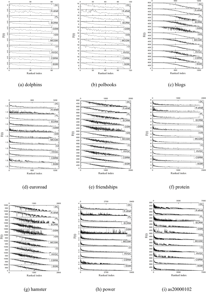
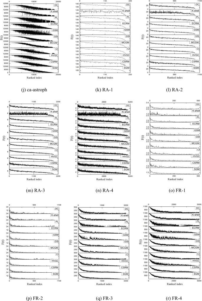
Stacked graphs of 11 algorithms on 18 datasets.

As depicted in Fig. 6, all the algorithms display an overall decreasing trend in their curves. However, algorithms with smoother and less fluctuating curves demonstrate closer alignment with the actual contagion dynamics. Specifically, on networks such as friendships, SGM showcases the fewest small spikes and exhibits smoother waveforms compared to other algorithms, indicating optimal performance on the network. On the hamster, as20000102, FR-3, and FR-4 datasets, both SGM and CSRM demonstrate superior performance with similar smoothness. On the dolphins, and ca-astroph networks, SGM shows slightly more volatility than the MCGM algorithm, yet it outperform other algorithms in terms of overall performance. Similarly, on the euroroad dataset, SGM and PL algorithms rank the highest, showcasing a consistently decreasing trend and the least number of small fluctuations in the waveforms. Regarding the protein, power, FR-1, FR-2 and four random networks, multiple algorithms, including SGM, demonstrate consistent performance.

Consistency of top-N nodes

Given the significance of the Top-N nodes with the highest influence within a network, Jaccard similarity can serve as a metric to evaluate the consistency of Top-N node selections by diverse algorithms compared to those identified through SIR models. Employing Eq. (23), a comparative analysis of similarity was conducted for 15 networks with over 400 nodes. This analysis involved progressively selecting the top 10 to 100 nodes, with the results depicted in Fig. 7. The proposed SGM algorithm demonstrates high performance across all but two networks, namely as20000102 and RA-2, where it exhibits moderate performance.

Fig. 7

Jaccard similarity of Top-N nodes.

Capacity differentiation of nodes

Based on the node ranking results obtained from each method and utilizing Eq. (22), the differentiation values in Table 5 are acquired. Remarkably, the proposed SGM algorithm demonstrates exceptional performance across all eleven networks: dolphins, polbooks, blogs, friendships, power, ca-astroph, RA-1, RA-2, RA-3, RA-4, and FR-3. Even on the seven other networks, although the differentiation values may not be the highest, each exceeds 0.94.

Table 5 Differentiation of node importance (retain three decimal places).

Ablation studies

To assess the significance of each component within the SGM algorithm model, an ablation study was conducted. This involved systematically removing specific components and observing the resulting changes in Kendall’s correlation coefficients. ‘SGM’ refers to the algorithm model proposed in this paper, as defined by Eq. (15) to Eq. (19). ‘R-A’, ‘R-B’, ‘R–C’, ‘R-D’, and ‘R-E’ represent the results obtained after sequentially removing specific components, with each step building upon the previous one.

$$R - A = \sum\limits_{{j \in \zeta_{i} }} {\delta_{i} \left( {\frac{SC(i)SC(j)}{{ds_{i,j}^{2} }}} \right)},$$

(24)

$$R - B = \sum\limits_{{j \in \zeta_{i} }} {\frac{SC(i)SC(j)}{{ds_{i,j}^{2} }}},$$

(25)

$$R - C = \sum\limits_{{j \in \zeta_{i} }} {SC(i)SC(j)},$$

(26)

$$R - D = SC(i),$$

(27)

$$R - E = k(i).$$

(28)

The following analysis can be derived from Fig. 8:

• (1) ‘R-A’ represents a modification of ‘SGM’ by removing the average clustering coefficients and the correlation component. As discussed in Section "Shannon gravity model", this part of the SGM model aims to minimize the impact of neighboring nodes in networks with sparse connections. Introducing the influence of neighboring nodes in such scenarios could potentially hinder the accurate assessment of the target node’s influence. This is further confirmed by the analysis of the ‘R-D’. While ‘SGM’ performs comparably to ‘R-A’ on most non-sparse networks, it shows superior performance on five sparse networks, namely euroroad, protein, power, and FR-1, which are characterized by low edge density and average clustering coefficients. This demonstrates the effectiveness of incorporating $\eta_{G}$ into the model, particularly in the context of sparse networks.

• (2) ‘R-B’ further removes the gravitational coefficient $\delta_{i}$ compared to ‘R-A’. In most networks, the removal of the gravitational coefficient leads to a decrease in the Kendall’s $\tau$. In artificial random networks, the impact of removing the gravitational coefficient is not significant. This is because random networks are generated with a uniform probability of connection, resulting in the maximum and average k-shell values being very similar. As the gravitational coefficient $\delta_{i}$ is correlated with the k-shell value, the removal of this component has a relatively insignificant impact on random networks.

• (3) ‘R–C’ further eliminates the distance ds_i,j from the gravity model compared to ‘R-B’. It can be observed that ‘R–C’ has a significantly lesser impact than ‘R-B’ on most networks, highlighting the necessity of this part of the design.

• (4) ‘R-D’, compared to ‘R–C’, removes the effect of neighboring points SC(j). For most networks, the Kendall’s $\tau$ appears to decrease. However, in the case of sparse networks such as euroroad, protein, power, FR-1, and FR -2 (which have a low ratio of connected edges to nodes and small average clustering coefficients), ‘R-D’ performs better than ‘R–C’. This suggests that for sparse networks, including the influence of neighboring points leads to poorer results. However, due to the compensation factors in other parts of the model, the proposed SGM algorithm performs very close to or even better than ‘R-D’ on sparse networks.

• (5) ‘R-E’ differs from ‘R-D’ by removing the logarithmic component of the sum of first-order neighbor degree values of node i, retaining only the degree value component. A significant performance decrease is observed across all 18 networks, underscoring the effectiveness of the Shannon capacity design for nodes.

Fig. 8

Experiments on the ablation of SGM algorithmic models.

Case study

In recent years, the global impact of the COVID-19 pandemic has presented significant challenges. This study examines the efficacy of the SGM algorithm using the Epi-1 dataset²⁴, which consists of a network comprising 647 nodes linked by 4645 relational edges. The network’s structure, following modularization, is depicted in Fig. 9. It is noteworthy that, while virus propagation is inherently directional at any given moment, this paper adopts the approach of Shetty et al.²⁴ and considers a scenario where the virus can propagate bidirectionally. Consequently, Epi-1 is treated as an undirected and unweighted network.

Fig. 9

COVID-19 network diagram.

It is essential to identify individuals within the network who exert greater influence over the transmission of the virus, thereby curbing the spread of the epidemic. Hence, in this manuscript, the Top-20 nodes for each algorithm’s computational outcomes on Epi-1 are selected to infect other nodes, resulting in the eventual propagation pattern illustrated in Fig. 10 and Table 6. Given the substantial likelihood of COVID-19 transmission, the contagion probability in the simulation ranges widely from 0.05 to 0.5. Among these algorithms, SGM, CSRM, PL, and DC exhibit the most effective and approximate contagion effects. This is attributed to the fact that these four algorithms select essentially the same Top-20 ranked nodes, as shown in Table 7. The infectivity of algorithms such as ECRM, CI, GSI, and HVGC demonstrates a slightly lesser degree of effectiveness. Meanwhile, the algorithms GSM, k-shell, and MCGM are considered to be the least effective. As shown in Table 7, when the probability of contagion is set to 0.1, the Top-7 nodes (3855, 3856, 3857, 3858, 3859, 3860, 3861) identified by the SIR model consistently rank within the Top-20 nodes across all 11 algorithms. Hence, the substantial variance in the ultimate contagion size primarily arises from the notably distinct behavior of the remaining thirteen nodes. For example, in addition to the seven nodes previously mentioned, the remaining 13 nodes within the Top-20 identified by the SGM, CSRM, PL, and DC algorithms are as follows: 3073, 3075, 3079, 3756, 3757, 3758, 3759, 3760, 3916, 3091, 4550, 3176, and 3177. Furthermore, the Kendall’s correlation coefficients of the four algorithms, SGM, CSRM, PL, and DC, which exhibited identical performance in the Top-20 contagion scenario, were compared. The average $\tau$ values for the SGM, CSRM, PL, and DC algorithms, as the probability of contagion varied from 0.05 to 0.5, were found to be 0.7665, 0.6927, 0.6719, and 0.6727, respectively. These results indicate that SGM outperforms the other three algorithms in terms of Kendall’ correlation. Overall, the SGM algorithm introduced in this study proves proficient in identifying pivotal nodes crucial for propagating the COVID-19 network (Epi-1).

Fig. 10

Top-20 node contagion size on Epi-1 networks.

Table 6 The contagion size value of Top-20 node on Epi-1 networks.

Table 7 Top-20 nodes of various algorithms on Epi-1 network.

Conclusion

The examination of the actual network substantiates the intricate connection between a node’s significance and structural elements of the network, including its position and the proximity of its neighboring nodes within a two-hop radius. Furthermore, through the study of node characteristics, a similarity has been observed between the Shannon model used in communication and complex network node identification. It is conceivable to regard a target node within a complex network, along with its neighboring nodes within two hops, as a sub-network. The significance of the target node can be determined by evaluating the Shannon capacity of this sub-network. Based on this analysis, we proposed the Shannon Gravity Model (SGM), an algorithm that innovatively combines the Shannon theorem with the gravity model to identify important nodes within the network. The SGM and other comparative algorithms were evaluated using the SIR contagion model. The results confirm that the SGM algorithm outperformed other algorithms, demonstrating superior consistency with real contagion results. In our future research endeavors, we intend to explore the viability of the SGM algorithm on directed networks and further optimize its performance by considering the relevant properties inherent in the respective networks.

References

Barabási, A. L. & Gulbahce, N. Network medicine: A network-based approach to human disease. Nat. Rev. Genet. 12, 56–68 (2011).
Vatani, N. & Rahmani, A. M. Personality-based and trust-aware products recommendation in social networks. Appl. Intell. 53, 879–903 (2023).
Liu, X. G., Hong, Z. Y., Liu, J. & Lin, Y. Computational methods for identifying the critical nodes in biological networks. Brief. Bioinform. 21, 486–497 (2020).
Borge-Holthoefer, J. & Moreno, Y. Absence of infuential spreaders in rumor dynamics. Phys. Rev. E 85, 026116 (2012).
Xu, W. Z., Li, T. & Liang, W. F. Identifying structural hole spanners to maximally block information propagation. Inf. Sci. 505, 100–126 (2019).
Bai, Y., Liu, S. & Li, Q. Cost-aware deployment of check-in nodes in complex networks. IEEE Trans. Syst. Man Cybern. Syst. 52, 3378–3390 (2021).
Kazemzadeh, F., Safaei, A. A. & Mirzarezaee, M. Determination of influential nodes based on the Communities’ structure to maximize influence in social networks. Neurocomputing 534, 18–28 (2023).
Freeman, L. C. Centrality in social networks conceptual clarification. Soc. Netw. 1, 215–239 (1979).
Kitsak, M., Gallos, L. K. & Havlin, S. Identification of influential spreaders in complex networks. Nat. Phys. 6, 888–893 (2010).
Newman, M. E. J. A measure of betweenness centrality based on random walks. Soc. Netw. 27, 39–54 (2005).
Watts, D. J. & Strogatz, S. H. Collective dynamics of ‘small-world’ networks. Nature 393, 440–442 (1998).
Bonacich, P. & Lloyd, P. Eigenvector-like measures of centrality for asymmetric relations. Soc. Netw. 23, 191–201 (2001).
Brin, S. & Page, L. The anatomy of a large-scale hypertextual web search engine. Comput. Netw. ISDN Syst. 30, 107–117 (1998).
Zhang, J. H., Zhang, Q. S. & Wu, L. Identifying influential nodes in complex networks based on multiple local attributes and information entropy. Entropy 24, 293 (2022).
Zareie, A., Sheikhahmadi, A. & Jalili, M. Finding influential nodes in social networks based on neighborhood correlation coefficient. Knowl. Based Syst. 194, 105580 (2020).
Sheng, J. F., Dai, J. Y. & Wang, B. Identifying influential nodes in complex networks based on global and local structure. Phy. A 541, 123262 (2020).
Zhao, J., Wang, Y. C. & Deng, Y. Identifying influential nodes in complex networks from global perspective. Chaos Solitons Fract. 133, 109637 (2020).
Yu, Z. J., Shao, J. M., Yang, Q. L. & Sun, Z. J. Profitleader: Identifying leaders in networks with profit capacity. World Wide Web 22, 533–553 (2019).
Zhong, L. F., Gao, X. Y. & Zhao, L. A hybrid influence method based on information entropy to identify the key nodes. Front. Phys. 11, 1280537 (2023).
Morone, F. & Makse, H. A. Influence maximization in complex networks through optimal percolation. Nature 524, 65–68 (2015).
Ma, Y., Cao, Z. L. & Qi, X. Q. Quasi-Laplacian centrality: A new vertex centrality measurement based on Quasi-Laplacian energy of networks. Phy. A 527, 121130 (2019).
Zhao, S. Y. & Sun, S. W. Identification of node centrality based on Laplacian energy of networks. Phy. A 609, 128353 (2023).
Salavati, C. & Abdollahpouri, A. Ranking nodes in complex networks based on local structure and improving closeness centrality. Neurocomputing 336, 36–45 (2019).
Shetty, R. D., Bhattacharjee, S. & Dutta, A. GSI: An influential node detection approach in heterogeneous network using covid-19 as use case. IEEE Trans. Comput. Soc. Syst. 10, 2489–2503 (2023).
Wang, G., Alias, S. B. & Sun, Z. J. Influential nodes identification method based on adaptive adjustment of voting ability. Heliyon 9, e16112 (2023).
Yang, Q., Wang, Y. H. & Yu, S. B. Identifying influential nodes through an improved k-shell iteration factor model. Expert Syst. Appl. 238, 122077 (2024).
Ma, L. L., Ma, C. & Zhang, H. F. Identifying influential spreaders in complex networks based on gravity formula. Phy. A 451, 205–212 (2016).
Li, Z., Ren, T. & Ma, X. Q. Identifying influential spreaders by gravity model. Sci. Rep. 9, 8387 (2019).
Zhong, L. F., Gao, X. Y. & Zhao, L. Identifying key nodes in complex networks based on an improved gravity model. Front. Phys. 11, 1239660 (2023).
Li, S. Y. & Xiao, F. Y. The identification of crucial spreaders in complex networks by effective gravity model. Inf. Sci. 578, 725–749 (2021).
Yang, X. & Xiao, F. Y. An improved gravity model to identify influential nodes in complex networks based on k-shell method. Knowl. Based Syst. 227, 107198 (2021).
Ullah, A., Wang, B. & Sheng, J. F. Identification of nodes influence based on global structure model in complex networks. Sci. Rep. 11, 6173 (2021).
Li, Z. & Huang, X. Y. Identifying influential spreaders by gravity model considering multi-characteristics of nodes. Sci. Rep. 12, 9879 (2022).
Zhu, S. & Zhan, J. Identifying influential nodes in complex networks using a gravity model based on the H-index method. Sci. Rep. 13, 16404 (2023).
Sun, Z. J., Sun, Y. N. & Chang, X. F. Finding critical nodes in a complex network from information diffusion and Matthew effect aggregation. Expert Syst. Appl. 233, 120927 (2023).
Shannon, C. E. A mathematical theory of communication. Bell Syst. Tech. J. 27, 379–423 (1948).
Hu, H. F. & Sun, Z. J. Exploring influential nodes using global and local information. Sci. Rep. 12, 22506 (2022).
Kumar, S. & Panda, A. Identifying influential nodes in weighted complex networks using an improved WVoteRank approach. Appl. Intell. 52, 1838–1852 (2022).
Goel, R., Bonnetain, L. & Sharma, R. Mobility-based SIR model for complex networks: with case study Of COVID-19. Soc. Netw. Anal. Min. 11, 1–18 (2021).
Valencia, D. & Lillo, R. E. A Kendall correlation coefficient between functional data. Adv. Data. Anal. Classif. 13, 1083–1103 (2019).
Acknowledgements
This work is supported by the Science and Technology Research Project of the Science and Technology Department of Henan Province, China (Grant Nos. 252102210028, 242102210131, 242102210205, 232102210147, 222102310601), the Scientific Research Projects of Colleges and Universities in Henan Province of China under Grant (25A520040, 25A120008, 22B520027), the Youth Foundation of Pingdingshan University (PXY-QNJJ-202103), and the Open Foundation of State key Laboratory of Networking and Switching Technology (Beijing University of Posts and Telecommunications(SKLNST-2022-1-10)).
Author information
Authors and Affiliations
Contributions
Conceptualization, Zhang S. M., Sun Z. J.; Validation, Zhang S. M., Wang G., Hu H. F.; Data collection, Wang F. F., Sun X. Y.; Data Curation and Writing, Zhang S. M., Sun Z. J.
Corresponding author
Ethics declarations
Competing interests
The authors declare no competing interests.
Additional information
Publisher’s note
Springer Nature remains neutral with regard to jurisdictional claims in published maps and institutional affiliations.
Rights and permissions
Open Access This article is licensed under a Creative Commons Attribution-NonCommercial-NoDerivatives 4.0 International License, which permits any non-commercial use, sharing, distribution and reproduction in any medium or format, as long as you give appropriate credit to the original author(s) and the source, provide a link to the Creative Commons licence, and indicate if you modified the licensed material. You do not have permission under this licence to share adapted material derived from this article or parts of it. The images or other third party material in this article are included in the article’s Creative Commons licence, unless indicated otherwise in a credit line to the material. If material is not included in the article’s Creative Commons licence and your intended use is not permitted by statutory regulation or exceeds the permitted use, you will need to obtain permission directly from the copyright holder. To view a copy of this licence, visit http://creativecommons.org/licenses/by-nc-nd/4.0/.
About this article
Cite this article
Zhang, S., Sun, Z., Wang, G. et al. Identifying influential spreaders based on improving communication transmission model and network structure. Sci Rep 15, 9380 (2025). https://doi.org/10.1038/s41598-025-93387-6
Received:
Accepted:
Published:
Version of record:
DOI: https://doi.org/10.1038/s41598-025-93387-6
Keywords
This article is cited by
-
WCM-GCN: identifying influential spreaders using graph convolutional networks on weighted directed networks based on spreading properties
Knowledge and Information Systems (2026)
Identifying influential spreaders on weighted directed networks based on spreading properties
The Journal of Supercomputing (2025)