
Abstract
This paper investigates the seismic performance of four-limb concrete-filled steel tubular (CFST) lattice columns with different slenderness ratios (10.8, 10.8, 18.4, and 27.9) and axial load ratios (0.2, 0.3, 0.2, and 0.2), conducting horizontal low-cycle reciprocating load test. Based on the test results, an artificial neural network (ANN) is used to improve the prediction of the seismic performance of four-limb CFST latticed columns, considering ANN’s defects of low accuracy prediction and the poor fitting for the load, unload and extreme point of hysteresis curves, the sparrow search optimization algorithm (SSA) is adopted to optimize the ANN’s weights and thresholds. Quantum computations are proposed to improve the SSA’s iteration convergence and avoidance of local optima, and its convergence curve is compared to circle chaotic sparrow search algorithm and tent chaos sparrow search algorithm (Tent-CSSA). The damage variables are calculated and compared with the predicted results from the SSA, the sparrow search algorithm based on quantum computations and multi-strategy enhancement (QMESSA) and the test results based on the energy damage model and Park’s model. The results demonstrate that the load–displacement hysteresis curves of Specimen 1 and Specimen 2 are bow-shaped, which show a strong plastic capacity. The hysteresis curve of Specimen 3 appears in an inverse S-shape, which was due to the slip caused by the low bond strength between concrete and steel pipe. The hysteresis curve of Specimen 4 is pike-shaped, which has a high shear span ratio and obvious bending performance. QMESSA effectively optimizes the weights and thresholds of the ANN, and its predicted damage variables are consistent with those of the conventional damage model. This indicates that QMESSA can effectively predict the load–displacement hysteresis curves of four-limb CFST lattice columns under low-cycle reciprocating loading.
Introduction
The seismic design of buildings closely relates to safeguarding people and their property as an earthquake can cause enormous damage to a structure. The demand for a high-rise structure has increased the significance of this issue. Scholars have studied the seismic performance of structures1,2,3. For example, Vu et al.4 used axial variable load tests to investigate the effect of variable axial forces on the seismic performance of reinforced concrete (RC) columns. Liberatore et al.5 analysis emphasizes the directionality of damage, the relevance of the vertical component of seismic excitation and the significant inelastic rotation caused by the columns and puts forward suggestions for improving the seismic behaviour of these types of structures. Tan et al.6 conducted axial load tests to study the seismic performance of reinforced pre-embedded column bases. Wei et al.7 used pseudo-dynamic tests to research the seismic performance of CFST columns and ultra-high performance concrete (UHPC) slabs. Many authors have improved the seismic performance of columns in different ways8,9. Kawashima et al.10 used polypropylene fiber-reinforced cement composites (PFRC) to reduce the damage of the cover layer and core concrete of the square bridge column, the local buckling of the longitudinal bar and the deformation of the tie bar in the shaking table test. The damage is much smaller than that of ordinary reinforced concrete columns. Domestic and international research on CFST lattice columns focuses on axial compression performance, while their horizontal hysteresis performance is less studied. The main purpose of the low-cycle reciprocating loading test is to study the mechanical properties and damage mechanisms of the structure after being subjected to such loading simulating seismic effects. Therefore, in this paper, the seismic performance of four-limb CFST lattice columns is investigated by using the low-cycle reciprocating loading test. The impact of various slenderness ratios and axial compression ratios on the strength, stiffness, and ductility of four-limb CFST latticed columns is discussed.
Studies utilizing the ANN have been made in the field of civil engineering, which can evaluate the seismic performance of structures quickly and accurately. Prayoonwet et al.11 used a neural network to predict the shear capacity of the RC beams without shear reinforcement. Zhang et al.12 employed a neural network to predict and design the mechanical properties of curved beams. Liang et al.13 used the ANN to predict the nonlinear buckling forces of steel–concrete composite structures under axial loading. Jia et al.14 employed a neural network to analyze the seismic damage of a RC frame with shear wall for multidimensional performance limit states. Ahmed et al.15 used the stacked long and short-term memory neural networks to predict the seismic damage states of RC structures. Cosgun.16 used the machine learning (ML) to predict and evaluate the seismic performance of existing RC structures. Previous studies have demonstrated that the ANN can effectively solve certain civil engineering problems. CFST latticed columns have been widely used in high-rise buildings due to their excellent seismic performance and high load-bearing capacity. Some tests on such composite structures have been conducted to study their seismic performance17,18. However, few studies using the ANN have been made to investigate the seismic performance of four-limb CFST latticed columns. Therefore, in this paper, the ANN is utilized to study the seismic performance of four-limb CFST latticed columns. The ANN is a mathematical or computational model that mimics the structure and function of biological neural networks (animal neural systems) and is capable of approximating complex nonlinear relationships19. Scholars have applied the ANN in the field of civil engineering. Hammoudi et al.20 employed the ANN to predict the compressive strength of recycled concrete aggregates, which yielded higher prediction accuracy than other methods. Nguyen et al.20 proposed a deep neural network to predict the compressive strength of foam concrete. Moradi et al.21 used an ANN model to predict the structural damage to bridges after vehicle fires. Jesús et al.22 employed an ANN to develop a prediction model to predict the compressive strength of self-compacting concrete. Shamass et al. 24 proposed an ANN capable of predicting web buckling capacity under various geometric variables to establish a comprehensive and practical design model tool. Amiri et al.23 utilized the characteristics of a reference sample to propose an ANN prediction model which was developed to predict the mechanics and durability of concrete. However, all of these neural networks are prone to fall into the phenomenon of local optimization and converge slowly during training. When the training data is small, the traditional ANN is prone to overfitting26. SSA is a relatively new intelligent optimization algorithm with good global optimization capability, convergence rate, and stability24.
SSA has a powerful global search capability, which can effectively jump out of the local minima to find a better solution. Meanwhile, the SSA method has good adaptability to adaptively adjust the search strategy for dynamically changing problems. In addition, SSA converges faster than traditional optimization algorithms, thus reducing the time required to train the neural network. In this study, the SSA is adopted to optimize neural network weights and thresholds with the addition of an early warning mechanism. The added mechanism selects a portion of the population an early warning and once the danger is detected, it chooses to give up and search for the optimal value again, allowing the optimization process to find a better value. Many scholars have conducted extensive research on SSA, which has been applied to many different scenarios. Ma et al.28 combine SSA with several innovative mutation strategies, including Improved Tent Chaos Mutation (IT), Lévy Flight Mutation (LF), Elite Opposition-Based Learning Mutation (EOBL), and Variable Radius Mutation (VR), as well as combinations of these approaches, to present a series of novel SSA variants. Ouyang et al.25 proposed a learning sparrow search algorithm in which a lens reversal learning strategy is introduced in the discoverer phase, while improved sine and cosine bootstrapping mechanisms are applied in the follower phase. These improvements lead to a more refined search method for the discoverer, thus solving the problem of zero dependency of traditional intelligent optimization algorithms. The algorithm shows good performance on CEC 2017 and a variety of benchmark test functions, effectively improving the situation where the algorithm falls into local optimal solutions. Wu and Yuan30 introduced nonlinear inertial weights into the entrants’ update formula of the contestant can enhance the local exploration ability of the algorithm. In addition, incorporating Lévy flights into the vigilant sparrows’ update formula of the alert sparrow helps to avoid the algorithm from falling into a local optimal solution in the late iteration. Yan et al.26 proposed an improved sparrow search algorithm based on iterative local search (ISSA), which solves the defects of the sparrow search algorithm in terms of the current underutilization of individuals and the inefficiency of searching, to improve its overall search performance. Yang et al.27 developed a new adaptive sparrow search algorithm by introducing a chaotic mapping strategy, an adaptive weighting strategy and a t-distribution mutation strategy, which solves the problems of slow convergence and easy to fall into local optimal solutions that exist in the basic SSA. Existing studies have improved the performance of SSA to a certain extent and verified its effectiveness in various application areas, which provides an important reference for subsequent studies. However, these researches still have some shortcomings, and the improved algorithms face limitations in practical applications, such as insufficient optimization accuracy and inefficient search efficiency, which are in urgent need of further improvement. Significant potential remains for achieving new progress by absorbing ideas or formulas from other algorithms and optimizing them based on their iterative properties. In addition, studies on the proof of convergence of the algorithm based on the sparrow search framework are relatively scarce, and more detailed mathematical analysis and research on the convergence of the algorithm and the rationality of its search mechanism remains an important issue. Quantum computing utilizes the superposition state and entanglement properties of quantum bits, enabling parallel processing of large amounts of information searched by a group and significantly improving computational efficiency. In the initialization phase, chaotic mapping and quantum computing are combined to improve the quality of the initial population. To jump out of the local optimum and balance the exploration and exploitation capabilities of the algorithm, an enhanced search strategy is introduced in the iterative phase to improve the capabilities of the algorithm. In addition, an exact elimination strategy is proposed to accelerate population convergence and further balance the iterative phase of development and exploration. When dealing with high dimensional and complex spaces, quantum computing shows greater advantages over classical computers and can optimize the structure and parameters of ANNs more efficiently. To make the SSA have a better iteration rate, accuracy, and global optimization-seeking ability, this study optimizes the SSA by utilizing quantum computing to numerically attain higher capacity and faster training speed33. The iteration rate and accuracy of the SSA are further enhanced by using quantum computations and multi-strategy enhancement (QME) to optimize the SSA28. The optimal weights and thresholds obtained from the QMESSA optimization algorithm are then used to reassign the parameters of the ANN and improve the prediction accuracy of the load–displacement hysteretic curves of four-limb CFST latticed columns.
Overview of the test
Test equipment
The concrete latticed columns, which serves as the test prototype, has a free top and a bottom secured to the ground by strong bolts and concrete slabs. A 100T vertical jack is used to exert the vertical load at the top of the columns and a loading plate is installed under the jack to prevent localized damage to the columns. A 1000kN MTS actuator is used to apply horizontal tension with a bolt link to the columns. The test loading device and specimen structure are shown in Fig. 1a,b, the structural details of the specimen are shown in Fig. 1c.

Loading device and specimen configuration.
Specimen design
The Q235 (yield strength = 235 MPa) welded steel pipe with an external diameter of 86 mm and thickness of 1.5 mm is used as a limb for the latticed columns. The composite limb is made of Q235 seamless steel pipe with the outer diameter of 48 mm, wall thickness of 2.5 mm. The lengths of the four specimens, SCC1, SCC2, SCC3, and SCC4, are respectively 1200 mm, 1200 mm, 2100 mm, and 3000 mm and the cross-section is typically 386 mm × 386 mm. SCC1, SCC3, and SCC4 have the same axial compression ratio of 0.2, while SCC2 has an axial compression ratio of 0.3. The slenderness ratios are 10.8 (SCC1 and SCC2), 18.4 (SCC3), and 27.9 (SCC4). The main parameters of the specimens are listed in Tables 1 and 2.
Specimen loading system
The specimen is initially preloaded with a force of 0.4–0.6N by a hydraulic jack, allowing the specimen to enter in normal working conditions and to ensure that the instrument will work properly. After checking the possible problems, apply the design axial force to the specimen and maintain it steadily.
After applying the axial compression to the columns, a horizontal reciprocating load is applied to the specimen. As shown in Fig. 2, in the load control stage, the actuator applies horizontal loads (\(1F\),\(2F\),\(3F\)…) to the columns until it yields (Py is yield load), with each load level cycled once. In the displacement control stage, the actuator applies horizontal loads (\(1\Delta_{y}\), \(2\Delta_{y}\), \(3\Delta_{y}\)…) to the columns until it yields(\(\Delta_{y}\) is yield displacement), with each displacement level cycled three times.

Low-cycle reciprocating load loading system.
Each loading is maintained for 2–3 min to record test results and observe the specimen’s appearance. To measure the vertical load of the column, a force transducer of 1000 kN is installed at the top and the horizontal load is obtained from the data acquisition system. The average horizontal displacements are taken by a displacement meter at the column top, middle portion of each column limbs, column base, and column’s equal and symmetrical parts. The specimen is considered damaged and the test is terminated when the specimen load is lowered by 15%, the loading displacement reaches 1/200 of the specimen’s height, or the column base exhibits clear damage characteristics.
Test results
The load–displacement hysteretic curves of the four specimens obtained from low-cycle reciprocating loading tests are shown in Fig. 3. The hysteretic curves of Specimens SCC1 and SCC2 are in bow shape and relatively full, manifesting strong plastic capacity. The hysteretic curve of Specimen SCC3 (Fig. 3c) is in inverse S-shape and less full, probably due to the slip caused by the low bonding strength between concrete and steel pipe. The hysteretic curve of Specimen SCC4 (Fig. 3d) is close to a pike shape, with a high shear span ratio and obvious bending properties, which are affected by the slenderness ratio.

Load–displacement hysteretic curves of the specimens.
load–displacement skeleton curve
The skeleton curve, as shown in Fig. 4, is an envelope curve formed by connecting the peak points of each loading cycle in the load–displacement hysteresis curve. The slenderness ratios of specimens 1, 3 and 4 are 10.8, 18.4 and 27.9, respectively. The axial compression ratios of specimens 1 and 2 are 0.2 and 0.3, respectively.

Comparison of Load–Displacement Skeleton Curves.
CorrectFrom Fig. 4a, the ultimate loads of specimens 1,3 and 4 are 79.42 kN, 49.60 kN and 33.45 kN respectively, and the ultimate displacements are 72.21 mm, 84.00 mm and 140.63 mm respectively. As the slenderness ratio of specimens 1, 3, and 4 grows, the stiffness of the component in the elastic stage decreases, the horizontal bearing capacity decreases, the ultimate displacement increases, and the ductility of the component improves. From Fig. 4b, as the axial compression ratio of specimens 1 and 2 grows, it can be seen the influence of axial compression ratio on the seismic performance of specimens is concentrated in the failure stage. In the elastic stage, the stiffness of the two is not significantly different, and the skeleton curve is roughly coincident. In the failure stage, the slope of the failure stage increases slightly as the axial compression ratio increases.
QMESSA neural network model
Performance comparison of optimization algorithms
The ANN is a subset of ML and the core of deep learning. It is a mathematical or computational model that mimics the structure and function of a biological neural network, often used to estimate or approximate a function. The ANN consists of an input layer, one or more hidden layers, and an output layer. Each node is referred as an artificial neuron with the associated weight and threshold when connecting with another node. Neural networks are trained on training sets and their accuracy improves with time. Using an optimization algorithm to tune neural networks improves their accuracy, making them as the powerful tools in computer science and artificial intelligence.
The SSA is used to optimize the ANN. This algorithm optimizes a neural network by updating the best position of the sparrow and possesses a better global optimization search capability, fewer control parameters, and simpler implementation compared to the Firefly Algorithm (FA) and Particle Swarm Optimization (PSO). Table 3 lists the test functions used in this study to examine three optimization algorithms: FA, PSO, and SSA. The test results for unimodal benchmark functions F1 to F7 and multimodal benchmark functions F8 to F12 are shown in Fig. 5.

The convergence curves of SSA, PSO, and FA on the test functions.
As shown in Fig. 5, the SSA converges much faster than the PSO and FA under the tests of unimodal benchmark functions F1, F2, and F3. Under the test of unimodal benchmark function F2, the convergence curves of the PSO and FA flatten out in the later iterations, while the convergence curve of the SSA continues to decrease, indicating that the SSA has sufficient ability to avoid the local optimum. Under these tests of unimodal benchmark functions, the SSA embodies the continuous convergence and converges to the theoretical optimum, while the PSO and FA fall into a local optimum. For the multimodal benchmark functions F9, F10, and F11, the SSA converges significantly faster than the PSO and FA and reaches the theoretical optimum after 73 iterations, while the PSO and FA trap into a local optimum. The convergence rate of all three algorithms (PSO, FA, and SSA) is similar when tested under the multimodal benchmark function F12, but the convergence accuracy of the SSA is significantly higher than that of the PSO and FA. This shows that the SSA outperforms the FA and PSO in terms of convergence rate and has better convergence accuracy and global optimization capability.
Establishment of QMESSA model
The basic unit in quantum computing is the quantum state. The quantum computing can solve some nondeterministic polynomial (NP) problems encountered in classical computing by using superposition, entanglement, and interference. QME is an algorithm solves the classical computational problem of factorization of large numbers and for random database searches to accelerate searches of unorganized databases. Because of its unique computing performance, the quantum computing based algorithm has quickly become a research hotspot. In the process of optimizing the SSA using quantum computing, quantum logic gates are used to realize the update operation of sparrow individuals for optimization. As shown in Fig. 6, the flow chart of QME optimized SSA-ANN neural network.

The flowchart of QME optimized SSA-ANN. ("0" and "1" denote the two respective basic states of quantum bits; φ denotes the superposition of quantum states, and α and β are the respective probability amplitudes of being in one of the two states).
In a quantum space, \(\left| {\left. 0 \right\rangle } \right.\) and \(\left| {\left. 1 \right\rangle } \right.\) are used to denote the two basic states of quantum bits, they make up the basic storage unit. Unlike classical computations, quantum bits can be in superposition of the two states simultaneously. The specific instruction is given as follows.
where φ denotes the superposition form of the quantum state by Eq. (2) and α and β represent the probability amplitudes of being in one of the two states, respectively.
In quantum computing, when quantum bits undergo a measurement, their state changes, which is known as the collapse. Before observation or measurement, a qubit is in a superposition state, meaning that it is in multiple potential states simultaneously. However, when measuring a quantum bit, it collapses into one of the definite states, while the other potential states disappear.
When a quantum state in a superposition state is observed, it collapses to zero with the probability \(\alpha^{2}\) or probability \(\beta^{2}\) (≤ 1). Depending on the probability amplitude, a quantum bit can be represented by a matrix form of sines and cosines, expressed as:
where cos θ = α and sin θ = β.
Quantum properties are applied to the population initialization process of the SSA. In this process, quantum bits are used to construct the individuals, with the probability amplitude representing the position of an individual. As a result, there is a correspondence between the quantum space position of an individual and the state matrix, as:
where xi,c represents the cosine position, xi,s represents the sine position, and \(\theta_{i,j}\) is the rotation angle (i = 1, 2, …, N, j = 1, 2, … , D).
The mapping relation between quantum space and solution space is established by the linear transformation. Suppose there exists a quantum bit \(\left[ {\cos \hat{I},\sin \hat{I}} \right]^{T}\) with values in the range [− 1,1] and the corresponding solution is [xc, xs]T with values in the range [lb, ub]. Next, the following transformation can be performed:
The position of each individual is determined by an improved circle chaotic mapping, so to correspond the quantum state collapses to a deterministic state after an observation. In order to regain the superposition state, the current state is assumed to be either a sine or cosine position and the inverse transformation is expressed by
By rotating the angle θ, the position corresponding to the other state can be decided. These two positions form the two state bits of the initial quantum bit.
In this study, a dynamic quantum rotation gate is used with the following formulation:
where \(\frac{\pi }{4} \le \theta_{r} \le \frac{\pi }{2}\). The update process of the dynamic quantum rotation gate is described by
The position of the population after mutation is determined according to Eqs. (5) and (6). By comparing the individuals at the initial and post-mutated sine and cosine positions, the optimal individuals are selected as the final initial population.
The adaptive T-distribution variation factor is formulated as follows:
The parentheses in Eq. (11) denotes the degrees of freedom, where t is the number of iterations, tc is the critical point in the iteration, and m is the scale factor (m = 10).
The steps of the SSA to optimize the neural network are described as follows.
-
1.
x1, x2,…, xm (m = 33) are the neural network input and y is the output (Fig. 7). Columns 1 to (n − 1) of the data are taken as the input, column n is taken as the output, and the data set is divided into training set and test set according to the ratio of 3:1.
Fig. 7 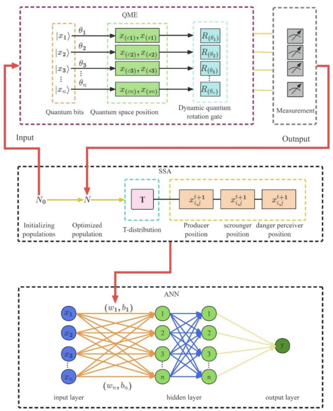
QMESSA-ANN prediction model.
-
2.
A feedforward neural network with 1, 2, …, n (n = 10) hidden layer nodes are constructed (Fig. 7). The neural network has two hidden layers and the network parameters are given. The training times are 1000, the training rate is 0.01, the training objective is 0.00001, the momentum factor is 0.01, the minimum performance gradient is 1e-6, and the number of maximum failures is 6.
-
3.
\(\left( {\omega_{1} ,{\text{b}}_{1} } \right)\), \(\left( {\omega_{2} ,{\text{b}}_{2} } \right)\), …, \(\left( {\omega_{n} ,{\text{b}}_{n} } \right)\) (n = 10) are the weights and thresholds of the neural network (Fig. 7). The weights and thresholds of the neural network are optimized using the SSA. For the parameters of the SSA, the number of populations is 30, the proportion of discoverers is 0.7, and the proportion of danger perceivers is 0.2.
In this paper, e.g., SCC1, 198,246 data samples are divided into training dataset, validation dataset and test dataset, where the test data are divided into two parts of validation dataset and test dataset in the ratio of 3:1. Figures 6 and 7 depict the flow of QME optimized SSA and the process of building the model is as follows.
-
I.
The first to penultimate columns are used as inputs (192888 samples) to train the neural network, and the last column is used as output (5358 samples), in which 75% of the samples (4018 samples) are used as validation neural network models, and 25% of the samples (1340 samples) are used as test neural network models. The number of neurons in the input layer usually corresponds to the dimension of the input feature, and the number of neurons in the output layer corresponds to the output dimension. The number of neurons in the input layers of SCC1, SCC2, SCC3, and SCC4 are 36, 48, 48, and 48, respectively, and the number of neurons in the output layer are all 1.
-
II.
Constructing ANN neural networks: The number of nodes in the hidden layer of the ANN neural network was set to 10. the number of training sessions was 1000, the learning rate was 0.01, the minimum error of the training objective was set to 0.00001, the display frequency was set to display once every 25 training sessions, the momentum factor was set to 0.01, and the maximum number of failures was set to 6. The tansig (hyperbolic tangent activation function) is the activation function used in the first layer (hidden layer), which has an output range of (-1, 1), and this function works well for nonlinear mapping of input values. The purelin (linear activation function) is an activation function used in the output layer, mainly for regression tasks, and its output is the same as the input with no nonlinear transformation. Its output range is \({( - \infty , + \infty })\). The loss function is the Mean Squared Error (MSE, Mean Squared Error). The formula is as follows:
$$MSE = \frac{1}{n}\sum\limits_{1}^{n} {(y_{i} - \hat{y}_{i} )}^{2}$$(12)where \(y_{i}\) is the true value, \(\hat{y}_{i}\) is the predicted value, and n is the sample size.
-
III.
Set the weights and thresholds of the neural network.
-
IV.
Setting the population size of this paper to 30, we chose the safety value ST=0.6 and the proportion of discoverers PD=0.7; the rest are followers. The proportion of sparrows aware of danger SD=0.2. (1). Calculate the fitness of each sparrow, in this paper the fitness is chosen as the mean square error of the test set. (2). The discoverer updates the position based on the current position and velocity. (3). Vigilant chooses a random location to explore to find a better solution. (4). The follower updates the position based on the current position and speed. (5). Repeat steps 1-4 until the termination condition is reached, i.e., the maximum number of iterations is reached. (6). Obtain the optimal weights and thresholds of the ANN neural network based on the optimal position.
-
V.
Build the T-distribution variance coefficient based on Eq. (11)
-
VI.
Update the positions of producer, scrounger, and danger perceiver.
-
VII.
Calculate the fitness of updated sparrow individuals.
-
VIII.
Record the current best weights and thresholds.
-
IX.
If the maximum number of iterations is not reached, return to construct probability amplitudes using quantum bits in the QME and reoptimize.
-
X.
If the maximum number of iterations is reached, output the optimal weights and thresholds.
-
XI.
Assign the optimal weights and thresholds to the ANN.
-
I.
-
4.
Train the neural network using the training data set.
-
5.
Error calculations are performed on the predicted results. The of MAE (Mean Absolute Error), RMSE (Root Mean Square Error), and MAPE (Mean Absolute Percentage Error) are calculated for the predicted and test results.

Predicted results and comparative analysis
QMESSA neural network predicted results
The QMESSA predicts the load–displacement hysteresis curves for the four specimens, and the errors are compared with the test results as shown in Table 4. In Fig. 8, the SSA and QMESSA are used to predict the four specimens. Figure 8a,b show excellent prediction results by the SSA and QMESSA, but as shown in Fig. 8c, at displacement of − 73.3 mm, the unload point (− 73.3, − 20.5), the loads of Specimen SCC3 predicted by both models increase, by 36.3% for the SSA and 29.7% for the QMESSA, compared to the test results. In Fig. 8d, at a displacement of 130.9 mm, the unloading point (130.9, 23.3), the load increase is 33.2% for the SSA and 11.3% for the QMESSA. These results show that the SSA optimization by the QME can improve the accuracy of the prediction model and the QMESSA can accurately predict the load–displacement hysteresis curve of CFST laced columns.

Predicted results of QME and SSA and test results.
The envelopes of the load–displacement hysteretic curves obtained from the SSA and QMESSA predictions and the tests are shown in Fig. 9. The skeleton curve can be divided into three stages:
-
(1)
Elastic stage. The load increases linearly with the displacement.
-
(2)
Strengthening stage. The load increases to a certain extent as the Poisson’s ratio of the steel pipe is smaller than that of the concrete, which generates a hoop effect, restraining the core concrete and increasing the specimen’s load capacity. However, the rate of load increase is slower than that in the elastic stage.
-
(3)
Degradation stage. Cracking appears in the limb tubes and the concrete at the column base is crushed, the load begins to decrease with increasing displacement.

Load–displacement skeleton curves.
CorrectThe trend of the predicted load–displacement envelope plots from the SSA and QMESSA is similar to that of the test results. The skeleton curves can reflect the effect of different parameters on the seismic performance of the specimens. The envelope plots obtained by the QMESSA are closer to the test results than those from the SSA, which is especially obvious in the case of reverse and forward loading. This indicates that the QMESSA can better predict the load–displacement hysteretic curve of four-limb CFST latticed columns.
The load–displacement hysteretic curves of Specimens SCC1, SCC3, and SCC4 are used as the training set, while the load–displacement hysteretic curve of Specimen SCC2 is used as the test set. The predicted results (red for the SSA and blue for the OMESSA) and test results (black) are shown in Fig. 8. As shown in Fig. 10a on the right side, the predicted result of SCC2 from the SSA is compared with the test result. In Fig. 10b on the right side, shows the predicted result of SCC2 from the QMESSA is compared with the test result. As seen from Fig. 10, both SSA and QMESSA predictions closely match the test results. At some stages of maximum loading, the QMESSA predictions are closer to the test results than the SSA predictions. For example, in steps 907, 924, and 940, the relative errors between the QMESSA predicted and test results are respectively 6.7%, 2.0%, and 1.1% for SCC2, respectively. The relative errors between the SSA prediction results and the test results are 8.9%, 4.8%, and 1.5%, respectively. It is obvious that the relative errors between the QMESSA model’s prediction results and the test results are smaller than those of the SSA model, which indicates that the prediction accuracy of the QMESSA model is higher.

Test results of SCC1, SCC3, and SCC4 and predicted results of SCC2.
CorrectPrediction for Tent-CSSA and CCSSA neural networks
To illustrate the applicability of the QMESSA for predicting the load–displacement hysteretic curve of four-limb CFST latticed columns, two other algorithms, Tent-CSSA and CCSSA are employed. The prediction error results of these two algorithms are compared. To ensure the reasonableness for the algorithm comparison, the following values are set: population size for all three prediction models = 30; the maximum number of iterations = 1000; number of training times = 1000; training rate = 0.01; and the minimum error of the training target = 0.00001.
As shown in Fig. 11, the load–displacement hysteretic curves predicted by the Tent-CSSA for SCC1 and SCC2 matchwell with the test results. However, the predicted curves for SCC3 and SCC4 different significantly from the test ones under the unloading condition: For SCC3, at a displacement of − 77.2 mm, the unload point (− 77.2, 27.0), the predicted load is 18.6% higher than the measured one; while for SCC4, at a displacement of 125.2 mm, the unload point (− 125.2, − 17.8), it increase by 37.6%.

Tent-CSSA predicted load–displacement hysteretic curves.
As shown in Fig. 12, the predicted load–displacement hysteresis curves for SCC1 and SCC2 by the CCSSA are in good agreement with the test results, whereas the predicted curves for SCC3 and SCC4 deviate significantly from the test results under the unloading state. For SCC3 with the load of − 20.51 kN, the unload point (− 75.1, − 20.5), the predicted displacement results increase by 11.8% compared to the test results; while for SCC4 with the load of -29.39kN, the extreme point (− 142, − 29.39), the displacement increase by 6.1%.

CCSSA predicted load–displacement hysteretic curves.
CorrectComparison of algorithm fitness
As shown in Fig. 13, among the four algorithms, the QMESSA has the highest convergence accuracy; while the Tent-CSSA has the lowest. The iteration rate of the four algorithms is higher at the beginning, the iteration curves of the SSA, Tent-CSSA, and CCSSA tend to become gentle after halfway of the iterations, while the convergence curve of the QMESSA continues to decline, indicating that the QMESSA has sufficient ability to escape from a local optimum. As depicted in Fig. 13a, the Tent-CSSA, SSA and CCSSA iterate respectively 365, 494, and 167 times of convergence stagnation and the convergence value of QMESSA has been declining, which indicates that the QMESSA can converge with higher accuracy. As shown in Fig. 13b, the Tent-CSSA and CCSSA iterate respectively 253 and 936 times of convergence stagnation. The convergence value of QMESSA and SSA continue to decline. The convergence accuracy of the QMESSA is higher than that of the other three algorithms. As depicted in Fig. 13c, the convergence stagnation of the CCSSA appears after 70 iterations. Before 227 iterations, the convergence accuracy of the CCSSA is higher than that of the QMESSA. After 227 iterations, the convergence accuracy of the QMESSA is higher than that of the CCSSA. As shown in Fig. 13d, the SSA, CCSSA, and Tent-CSSA iterate respectively 650, 408, and 531 times of convergence stagnation. The convergence curve of the QMESSA continues to decline and the convergence accuracy of the QMESSA is the highest. This shows that the QME can effectively optimize the SSA and improve the iteration speed and accuracy of the SSA.

Convergence curves of the QMSSA and other improved SSA.
Error results
The errors of the four algorithms (QMESSA, SSA, Tent-CSSA, and CCSSA) for predicting the load–displacement hysteresis curves of four-limbed CFST latticed columns are indicated in Table 4. Among the four algorithms, the QMESSA has the smallest MAE, RMSE, and MAPE, with the MAPE less than 5%, indicating that the QMESSA has the best predictive ability. As seen from Table 6, for SCC4, the MAE of the QMESSA is lower by 0.1033, 0.7941 and 0.4800, while the RMSE is reduced by 0.2565, 1.2202 and 0.9590, compared to the MAE of the SSA, Tent-CSSA, and CCSSA, respectively. As demonstrated, the QMESSA outperforms other algorithms in predicting the load–displacement hysteresis curves of four-limb CFST latticed columns.
Comparison with traditional methods
The energy damage model is used to calculate the damage variable (D) of a specimen under low cyclic loading, using the following formula:
where k0 is the average stiffness of the component in the positive and negative directions during the initial loading, \(\pm \Delta_{i}\) is the amount of deformation from the ith cycle of forward and reverse loadings to the maximum loading, and \(\int_{{\Delta_{0} }}^{{ \pm \Delta_{1} }} {ds}\) is the absolute integral of a displacement value to the maximum displacement when the load is 0 under the unipolar cyclic loading.
The deformation damage and energy dissipation damage can be determined using the Park29 model which is suitable for modeling the nonlinear behavior of reinforced concrete. The CFST latticed column is composed of concrete, reinforcing steel, and steel tube. Its structure and material composition are rather complex, thus difficult to use the traditional linear elastic model to accurately describe its nonlinear behavior. The two-parameter model considers the process of concrete compression and concrete tensile failure, as well as the damage accumulation effect of materials. Therefore, the Park model is used to calculate the damage variable of the specimen under low cyclic loading, using this formula:
where \(\delta_{m}\) is the maximum deformation; \(\delta_{u}\) is the ultimate deformation; \(\beta\) is the energy dissipation factor; \(\int {dE}\) is the hysteretic energy dissipation; \(Q_{y}\) is the calculated yield strength; \(\lambda\) is the shear-to-span ratio; \(n_{0}\) is the reinforcement rate of the longitudinal rebars in tension; and \(\rho_{w}\) is the volumetric stirrup ratio. The calculation parameters are listed in Table 5.
A comparison of cumulative energy consumptions is shown in Fig. 14. During the test, SCC1 and SCC2 show identical damage patterns. The column base of the limb tube tears when SCC1 is loaded to 60 mm, and the resulting cumulative energy dissipation is 59,329.8 N-mm (Fig. 14a). With SSC2 loaded to 72 mm, the concrete at the column bottom is crushed and the resulting cumulative energy dissipation is 51,326.3 N-mm (Fig. 14b). With SCC3 loaded up to 72 mm, there is a significant bulge at the column base, and the resulting cumulative energy dissipation is 28,757.9 N-mm (Fig. 14c). With SCC4 loaded to 150 mm, there is a significant bulge in the columns and the cumulative energy dissipation value is 66,142.8 N-mm (Fig. 14d). The calculated cumulative energy consumptions from the SSA and QMESSA prediction data follow the same trend as the test results and the cumulative energy consumptions obtained from the QMESSA prediction data are closer to the test results than those obtained from the SSA prediction data (Fig. 14). This indicates that the QMESSA has a better prediction and that the QME can effectively optimize the SSA.

True cumulative energy consumption and specimen failure phenomena and machine learning (ML) predicted results.
In Eq. (14), when β is 0.10, the Park’s formula is Park1 and when β is 0.15, the Park’s formula is Park2. The test damage variables for the four specimens are calculated separately using the damage model and Table 8 lists the calculation results. The traditional damage model is used to calculate the damage variable of the ML predicted data based on the damage state of the four specimens. Due to the accumulation of damages during the test, the ultimate deformation of the specimens under monotonic loading exceeds the maximum displacement. The monotonic loading ultimate displacement divided by 0.62 corresponds to the value of \(\delta_{u}\) in the damage state36. The damage variables from the ML are indicated in Table 7.
A comparison of damage variables between the predicted results by the ML and the test results calculated by the energy damage model and Park model (Tables 6 and 7) is presented in Fig. 15. As observed, the test results are close to the ML predictions, indicating that the data obtained from the QMESSA prediction fit the test results better, with the smallest difference of 0.7477 between the test results and the ML prediction results, in Specimen SSC3. This manifests that the QMESSA can be applied to predict the load–displacement hysteretic curve of four-limb CFST latticed columns.

Comparison of damage variables (Note: D, DP1, and DP2 real values are the damage variables calculated from the test results using the Park model and energy damage model; D, DP1, and DP projected values are the damage variables obtained from the neural network prediction data using the Park model and energy damage model).
The relative errors between the traditional damage model and the ML damage results are listed in Table 8. As indicated, the maximum relative error is under 5%, indicating that the QMESSA can accurately predict the load–displacement hysteretic curve of four-limb CFST latticed columns and that it is feasible to utilize the QMESSA prediction results to determine the damage variables.
Conclusions
This study aims to predict the load–displacement hysteresis curves of four-limb concrete-filled steel tubular (CFST) latticed columns under low-cyclic reciprocating loading tests. Aiming at the problem of low prediction accuracy and poor fitting at the load, unload and extreme point of hysteresis curve, quantum computations and multi-strategy enhancement (QME) improved sparrow search optimization algorithm (SSA) is used to optimize the neural network. The damage model is applied to calculate the damage variables from the test and predicted results separately. According to this study, the following major findings are offered:
-
(1)
The fullness and shape of load–displacement hysteretic curves are influenced by the longitudinal rebar’s reinforcement rate and shear-to-span ratio factors. With the increase of the slenderness ratio of specimens 1, 3, and 4, the ultimate displacements of specimens 3 and 4 increased by 16.33% and 94.75%, respectively, compared to specimen 1, but the horizontal ultimate loads fell by 37.55% and 57.88%. The results show that a higher slenderness ratio reduces horizontal load-bearing capacity, increases ultimate displacement, and improves specimen ductility. As the axial load ratio increases, the slope during the failure phase rises slightly.
-
(2)
The cumulative energy consumptions of the QMESSA prediction data are closer to the cumulative energy consumptions of the test results than those from the SSA, and the skeleton curves of the machine learning prediction data are closer to the measured ones than those from the SSA. The machine learning damage results match generally well with those of the traditional model, with the maximum error under 5%, demonstrating a high precision. It also shows that the QME can effectively optimize the SSA and improve the prediction accuracy of the SSA, while the QMESSA can effectively predict the load–displacement hysteretic curve of four-limb CFST latticed columns.
-
(3)
The SSA performs better than Particle Swarm Optimization (PSO) and Firefly Algorithm (FA) in terms of convergence rate, convergence accuracy, and global optimization ability for the 12 test functions considered. The QMESSA has the fewest iterations and highest accuracy compared to the SSA, tent chaos sparrow search algorithm (Tent-CSSA), and circle chaotic sparrow search algorithm (CCSSA). This shows QME can improve the iterative accuracy and speed of SSA.
-
(4)
The comparison of SSA MAE, RMSE, and MAPE results shows that the QMESSA’s prediction errors are small, indicating that the SSA is well optimized by the QME in predicting the load–displacement hysteresis curves of four-limb CFST latticed columns.
Data availability
The datasets used and/or analysed during the current study available from the corresponding author on reasonable request.
References
Han, Y. & Bao, Y. H. Seismic performance of steel-reinforced concrete-filled rectangular steel tubes after exposure to non-uniform fire. Sci. Rep. 13, 1322. https://doi.org/10.1038/s41598-023-28517-z (2023).
Pang, X. & Li, Y. Seismic performance evaluation of precast post-tensioned high-performance concrete frame beam-column joint under cyclic loading. Sci. Rep. 14, 12327. https://doi.org/10.1038/s41598-024-63083-y (2024).
Khan, M. S. Seismic behavior of SMA-reinforced ECC columns under different axial load ratios. Iran J. Sci. Technol. Trans. Civ. Eng. 47, 2295–2309. https://doi.org/10.1007/s40996-023-01049-2 (2023).
Vu, N. S. & Li, B. Seismic performance of flexural reinforced concrete columns subjected to varying axial forces. Eng. Struct. 310, 118090. https://doi.org/10.1016/j.engstruct.2024.118090 (2024).
Liberatore, L., Sorrentino, L., Liberatore, D. & Decanini, L. D. Failure of industrial structures induced by the Emilia (Italy) 2012 earthquakes. Eng. Fail. Anal. 34, 629–647. https://doi.org/10.1016/j.engfailanal.2013.02.009(2013) (2012).
Tan, S. S., Guo, L. H., Jia, C. & Xu, Y. Experimental investigation on seismic performance of an enhanced embedded base for CFST columns. Eng. Struct. 300, 117154. https://doi.org/10.1016/j.engstruct.2023.117154 (2024).
Wei, J. G. et al. Seismic performance of concrete-filled steel tubular composite columns with ultra high performance concrete plates. Eng. Struct. 278, 115500. https://doi.org/10.1016/j.engstruct.2022.115500 (2023).
Khan, M. S. Seismic performance of deficient RC frames retrofitted with SMA-reinforced ECC column jacketing. Innov. Infrastruct. Solut. 6, 157. https://doi.org/10.1007/s41062-021-00529-6 (2021).
Basit, A., Khan, M. S. & Ahmad, N. Rehabilitation of reinforced concrete frames with non-seismic details using eccentric steel braces. Struct. Eng. Mech. 80(4), 401–416. https://doi.org/10.12989/sem.2021.80.4.401 (2021).
Kawashima, K. et al. Seismic performance of a full-size polypropylene fiber-reinforced cement composite bridge column based on E-defense Shake table experiments. J. Earthq. Eng. 16(4), 463–495. https://doi.org/10.1080/13632469.2011.651558 (2012).
Prayoonwet, W. et al. Shear strength prediction for RC beams without shear reinforcement by neural network incorporated with mechanical interpretations. Eng. Struct. 298, 117065. https://doi.org/10.1016/j.engstruct.2023.117065 (2024).
Zhang, J. H. & Xue, X. Mechanical properties prediction and design of curved beams by neural network. Thin-Wall. Struct. 195, 111434. https://doi.org/10.1016/j.tws.2023.111434 (2024).
Liang, Z. T., Zhao, Y. Y., Yu, H. W., Habibi, M. & Mahmoudi, T. Artificial neural networks coupled with numerical approach for the stability prediction of non-uniform functionally graded microscale cylindrical structures. Structures 60, 105826. https://doi.org/10.1016/j.istruc.2023.105826 (2024).
Jia, D. W. & Wu, Z. Y. Seismic fragility analysis of RC frame-shear wall structure under multidimensional performance limit state based on ensemble neural network. Eng. Struct. 246, 112975. https://doi.org/10.1016/j.engstruct.2021.112975 (2021).
Ahmed, B., Mangalathu, S. & Jeon, J. S. Seismic damage state predictions of reinforced concrete structures using stacked long short-term memory neural networks. J. Build. Eng. 46, 103737. https://doi.org/10.1016/j.jobe.2021.103737 (2022).
Cosgun, C. Machine learning for the prediction of evaluation of existing reinforced concrete structures performance against earthquakes. Structures 50, 1994–2003. https://doi.org/10.1016/j.istruc.2023.02.127 (2023).
Huang, Z., Jiang, L. Z., Chen, Y. F., Luo, Y. & Zhou, W. B. Experimental study on the seismic performance of concrete filled steel tubular laced column. Steel Compos. Struct. 26(6), 719–731. https://doi.org/10.12989/scs.2018.26.6.719 (2018).
Feng, Y. L. et al. Calculation method and application of natural frequency of integrated model considering track-beam-bearing-pier-pile cap-soil. Steel Compos. Struct. 49(1), 81. https://doi.org/10.12989/scs.2023.49.1.081 (2023).
Wang, J., Zhai, Y. L., Yao, P. T., Ma, M. Y. & Wang, H. Established prediction models of thermal conductivity of hybrid nanofluids based on artificial neural network (ANN) models in waste heat system. Int. Commun. Heat Mass Transf. 110, 104444. https://doi.org/10.1016/j.icheatmasstransfer.2019.104444 (2020).
Hammoudi, A. et al. Comparison of artificial neural network (ANN) and response surface methodology (RSM) prediction in compressive strength of recycled concrete aggregates. Constr. Build. Mater. 209, 425–436. https://doi.org/10.1016/j.conbuildmat.2019.03.119 (2019).
Nguyen, T. et al. Deep neural network with high-order neuron for the prediction of foamed concrete strength. Computer-Aided Civ. Infrastruct. Eng. 34(4), 316–332. https://doi.org/10.1111/mice.12422 (2019).
Mohammad, J. M., Gita, M., Masoud, A. & Hamzeh, H. Structural damage levels of bridges in vehicular collision fires: Predictions using an artificial neural network (ANN) model. Eng. Struct. 295, 116840. https://doi.org/10.1016/j.engstruct.2023.116840 (2023).
Jesús, D. P. G. et al. To determine the compressive strength of self-compacting recycled aggregate concrete using artificial neural network (ANN). Ain Shams Eng. J. 15(2), 102548. https://doi.org/10.1016/j.asej.2023.102548 (2024).
Rabee, S., Felipe, P. V. F., Vireen, L., Luis, F. P. S. & Konstantinos, D. T. Web-post buckling prediction resistance of steel beams with elliptically-based web openings using Artificial Neural Networks (ANN). Thin-Wall. Struct. 180, 109959. https://doi.org/10.1016/j.tws.2022.109959 (2022).
Mostafa, A. & Farzad, H. Prediction of mechanical and durability characteristics of concrete including slag and recycled aggregate concrete with artificial neural networks (ANNs). Constr. Build. Mater. 325, 126839. https://doi.org/10.1016/j.conbuildmat.2022.126839 (2022).
Asteris, P. G. & Mokos, V. G. Concrete compressive strength using artificial neural networks. Neural Comput. Appl. 32(15), 11807–11826. https://doi.org/10.1007/s00521-019-04663-2 (2022).
Zhang, Z. Z., Li, K., Guo, H. Y. & Liang, X. Combined prediction model of joint opening-closing deformation of immersed tube tunnel based on SSA optimized VMD, SVR and GRU. Ocean Eng. 305, 117933. https://doi.org/10.1016/j.oceaneng.2024.117933 (2024).
Ma, B. et al. Enhanced sparrow search algorithm with mutation strategy for global optimization. IEEE Access 9, 159218–159261. https://doi.org/10.1109/ACCESS.2021.3129255 (2021).
Ouyang, C., Zhu, D. & Wang, F. A learning sparrow search algorithm. Comput. Intell. Neurosci. 1, 3946958. https://doi.org/10.1155/2021/3946958 (2021).
Wu, D. & Yuan, C. Threshold image segmentation based on improved sparrow search algorithm. Multimed. Tools Appl. 81(23), 33513–33546. https://doi.org/10.1007/s11042-022-13073-x (2022).
Yan, S., Yang, P., Zhu, D., Zheng, W. & Wu, F. Improved sparrow search algorithm based on iterative local search. Comput. Intell. Neurosci. 2021(1), 6860503. https://doi.org/10.1155/2021/6860503 (2021).
Yang, X. et al. A novel adaptive sparrow search algorithm based on chaotic mapping and t-distribution mutation. Appl. Sci. 11(23), 11192. https://doi.org/10.3390/app112311192 (2021).
Abbas, A. et al. The power of quantum neural networks. Nat. Comput. Sci. 1(6), 403–409. https://doi.org/10.1038/s43588-021-00084-1 (2021).
Wu, R. et al. An improved sparrow search algorithm based on quantum computations and multi-strategy enhancement. Expert Syst. Appl. 215, 119421. https://doi.org/10.1016/j.eswa.2022.119421 (2023).
Ni, W. B. et al. Estimation and analysis of the cumulative energy damage model for precast concrete nonrectangular column frame structures. Structures 58, 105529. https://doi.org/10.1016/j.istruc.2023.105529 (2023).
The international federation for structural concrete CEB-FIP displacement-based seismic design of reinforced concrete buildings. Lausanne Switzerland: The International Federation for Structural Concrete (2003).
Acknowledgements
The authors would like to express their gratitude for the financial support provided by National Natural Science Foundation of China (Grant No. 52204210, 51808213), Natural Science Foundation of Hunan Province, China (Grant No. 2023JJ30242, 2019JJ50185), Research Foundation of Education Bureau of Hunan Province, China (Grant No. 21B0452, 20B214), and China Scholarship Council. The opinions expressed in this paper are solely of the authors, however.
Author information
Authors and Affiliations
Contributions
Juan Chen: Writing-review and editing, Project administration, Funding acquisition; Jun-Jie He: Original-draft writing; Investigation, Data processing; Zhi Huang: Conceptualization, Methodology, Supervision, Project administration; Yuner Huang: Conceptualization, Methodology, Supervision; Y. Frank Chen: Comments and proofreading.
Corresponding author
Ethics declarations
Competing interests
The authors declare no competing interests.
Additional information
Publisher’s note
Springer Nature remains neutral with regard to jurisdictional claims in published maps and institutional affiliations.
Rights and permissions
Open Access This article is licensed under a Creative Commons Attribution-NonCommercial-NoDerivatives 4.0 International License, which permits any non-commercial use, sharing, distribution and reproduction in any medium or format, as long as you give appropriate credit to the original author(s) and the source, provide a link to the Creative Commons licence, and indicate if you modified the licensed material. You do not have permission under this licence to share adapted material derived from this article or parts of it. The images or other third party material in this article are included in the article’s Creative Commons licence, unless indicated otherwise in a credit line to the material. If material is not included in the article’s Creative Commons licence and your intended use is not permitted by statutory regulation or exceeds the permitted use, you will need to obtain permission directly from the copyright holder. To view a copy of this licence, visit http://creativecommons.org/licenses/by-nc-nd/4.0/.
About this article

Cite this article
Chen, J., He, JJ., Huang, Z. et al. Four-limb CFST latticed columns seismic performance: experimental and ANN predictions. Sci Rep 15, 33030 (2025). https://doi.org/10.1038/s41598-025-99328-7
Received:
Accepted:
Published:
Version of record:
DOI: https://doi.org/10.1038/s41598-025-99328-7
