A multi-branch network for cooperative spectrum sensing via attention-based and CNN feature fusion

Abstract

In cognitive radio (CR) systems, the accurate detection of spectrum holes is a cornerstone for efficient spectrum utilization. However, the increasing complexity of CR environments, particularly those with multiple primary users (PUs), has made precise spectrum sensing a paramount challenge. To address this challenge, this study introduces the ATC model, a novel deep learning architecture that integrates a parallel combination of attention mechanism-based networks and a Convolutional Neural Network (CNN). This hybrid design enables the model to capture both spatial and temporal features from the distinct statistics of sensing signals, thereby enhancing the accuracy of spectrum state detection. The model employs a Graph Attention Network (GAT) to extract complex topological features from graph-structured data derived from received signal strength, dynamically highlighting the most relevant information. To complement this, a CNN processes the sample covariance matrix of sensing signals, unlocking localized statistical correlations and hierarchical feature representations by treating the matrix as an image. Temporal dynamics, such as PU activity patterns, are modeled using a Transformer encoder, which leverages a self-attention mechanism to learn sequential features effectively. The proposed model is evaluated using both simulated and real-world datasets. For the simulated datasets, the model is assessed and compared with baseline methods under multi-PU scenarios across different channel models. For the real-world dataset, the experimental setup is configured for a single-PU scenario due to practical data collection limitations. In both cases, the ATC model demonstrates improved performance over the benchmarked spectrum sensing methods, exhibiting higher accuracy and robustness within the respective evaluation settings.

Introduction

The increasing demand for radio frequency spectrum, driven by the rapid expansion of wireless communication systems and the Internet of Things (IoT), faces a significant challenge: spectrum scarcity. Cognitive radio networks (CRNs) offer a promising solution by enabling dynamic spectrum access, allowing unlicensed secondary users (SUs) to opportunistically utilize spectrum bands not currently occupied by licensed primary users (PUs)^1,2,3.

Effective spectrum sensing is paramount in CRNs. It enables SUs to identify these ”spectrum holes,” maximizing spectrum utilization while minimizing interference with PUs. While single-SU sensing is susceptible to channel impairments like fading, cooperative spectrum sensing (CSS), where multiple SUs collaborate, offers improved detection reliability^4,5.

Recent research has explored machine learning (ML) for enhanced spectrum sensing^6,7. Traditional ML approaches, such as k-Nearest Neighbor (kNN), K-means, and Support Vector Machines (SVM), have been applied to classify spectrum occupancy based on learned signal features^8,9,10,11. However, deep learning (DL) has demonstrated superior performance in extracting complex signal characteristics. Studies have successfully employed neural networks like Convolutional Neural Network (CNN)^12,13,14,15, Long Short-Term Memory network (LSTM)^16,17, and Graph Convolutional Network (GCN)¹⁸ for single-PU spectrum sensing, capturing both spatial and temporal signal features.

A significant limitation of existing spectrum sensing methods is their primary focus on single-PU scenarios, while the more complex scenario with multiple PUs remains largely unaddressed. This is particularly relevant in power-domain Non-Orthogonal Multiple Access (NOMA) networks, where multiple users are permitted to utilize the same channel with distinct power levels. Accurate sensing of the PU channel status enables SU systems to exploit available spectrum holes, thereby improving the efficiency of overall spectrum utilization. In cellular networks, multiple PUs in adjacent cells may operate on the same frequency band. In this scenario, SUs are required to precisely sense the channel status of all active PUs. This ensures efficient frequency reuse across both time and space.

This work addresses the above challenge by proposing a novel framework, the ATC model, for spectrum sensing in multi-PU CRNs. The ATC model not only detects the presence of active PUs but also identifies which PUs are active, enabling SUs to optimize their spectrum access strategies. The proposed model is designed to integrate the learned features of the received signals by systematically exploiting their diverse statistical characteristics. The ATC model consists of the following key components:

Graph Attention Network (GAT): The GAT exploits complex spatial characteristics among SUs by leveraging the received signal strength (RSS). Unlike traditional GCNs that assign fixed weights to neighboring nodes, the GAT employs the attention mechanism to dynamically weight neighboring SU contributions based on their relevance^19,20. This enables more effective modeling of inter-SU spatial dependencies based on RSS information.

Covariance Matrix (CM) and CNN: To further enrich the spatial feature representation, we utilize the sample CM of the received signals, which provides robust second-order statistics and is less sensitive to noise¹⁵. A CNN is then applied to the CM, allowing the model to capture fine-grained spatial structures and statistical correlations in the sensing signals. This design complements the GAT by extracting spatial features from a different statistical perspective.

Transformer Encoder: To capture the temporal dynamics of PU activity, a Transformer encoder is employed. Its self-attention mechanism excels at capturing long-range dependencies in sequential data, providing a more effective approach for learning PU activity patterns compared to recurrent networks like LSTM²¹.

The proposed model is evaluated on both synthetic and real-world datasets across various scenarios. Experimental results demonstrate its superior performance in spectrum sensing compared to existing models.

In summary, the paper’s contributions are as follows:

• This work addresses the CSS problem in CRNs with multiple PUs. The proposed CSS framework enhances spectrum utilization by accurately identifying active PUs, as validated by experimental results.

• The proposed model is designed to effectively learn complex spatial representations by employing GAT and CNN on diverse statistics. In addition, a Transformer encoder is utilized to capture temporal dependencies by modeling the sequential dynamics of the received signal data.

• To evaluate the proposed model, synthetic and real-world datasets are used in this work. Specifically, the synthetic datasets are used to validate the performance improvement over existing methods under multi-PU scenarios. Due to practical data collection limitations, the real-world dataset is employed to evaluate the model performance under the single-PU scenario. The experimental results demonstrate that the proposed model outperforms the benchmarked methods within the considered evaluation scenarios.

The remainder of this paper is structured as follows. Section II reviews the background and related works on CSS algorithms. Section III presents the problem formulation, while Section IV details the proposed methodology. Experimental results are analyzed in Section V, followed by conclusions in Section VI.

Background and related works

The field of spectrum sensing has evolved significantly alongside the growth of CRNs, offering innovative solutions to address the challenge of spectrum scarcity. This section reviews existing spectrum sensing techniques, highlighting their strengths and limitations-especially in environments with multiple PUs-underscoring the need for advanced approaches.

Spectrum sensing techniques in CRNs

Traditional methods

Traditional spectrum sensing methods, such as energy detection, matched filter detection, and cyclostationary feature detection, have inherent limitations. Energy detection is susceptible to noise and performs poorly in low signal-to-noise ratio (SNR) environments, making it unreliable in many real-world scenarios^22,23. Matched filter detection, while more effective, requires prior knowledge of the primary user signals, which limits its applicability in dynamic or unpredictable settings²⁴. Cyclostationary feature detection leverages signal periodicity but introduces high computational complexity, making it less practical for large-scale networks²⁵.

Cooperative spectrum sensing (CSS)

Cooperative Spectrum Sensing has emerged as a promising approach to enhance detection reliability by aggregating observations from multiple SUs. Hard decision fusion schemes, such as majority voting, reduce bandwidth overhead but discard valuable soft information. In contrast, soft-fusion methods preserve signal details but increase communication overhead^26,27. Despite these improvements, traditional CSS methods often struggle with heterogeneous channel conditions and scalability in dense networks.

Recent advancements propose semi-soft decision schemes and efficient soft decision fusion rules to balance sensing performance with communication overhead^28,29. Furthermore, studies evaluating transmitter detection techniques (e.g., energy detection, matched filter, and cyclostationary feature detection) highlight both their practical utility and limitations in realistic deployments^30,31.

Machine learning for spectrum sensing

Early machine learning approaches

Initial methods employed algorithms such as SVM and k-NN, using hand-crafted features like energy statistics and spectral correlations. SVM-based classifiers demonstrated moderate accuracy in static conditions; however, their reliance on manually engineered features and assumptions about noise limited effectiveness in dynamic environments¹¹. Similarly, k-NN classifiers faced challenges with high-dimensional data and computational inefficiency, affecting their scalability and performance in complex spectrum sensing tasks⁸.

Advancements with deep learning

The advent of deep learning introduced models capable of automatically extracting intricate signal features, enhancing spectrum sensing capabilities. Convolutional Neural Networks (CNNs) capture spatial patterns from time-frequency representations such as spectrograms, leading to improved detection rates¹³. Recurrent Neural Networks (RNNs), including LSTM and GRU, adeptly model temporal dependencies in time-series data, facilitating robust sensing in fading channels³². Graph Convolutional Networks (GCNs) exploit the topological structure of SU networks to enhance decision fusion in CSS^18,33.

Recently, hybrid deep learning architectures have emerged. CNN-LSTM models enhanced with channel attention improve robustness in cooperative sensing under varying conditions³⁴. CNN-Transformer (CNN-TE) hybrids capture both local structures and long-range dependencies in sensing signals³⁵.

Limitations and Challenges: Despite these advances, most models are tailored for single-PU detection. Applying them to multi-PU environments often degrades performance, as they may fail to capture cross-PU correlations or prioritize discriminative features across diverse signals. Traditional non-deep methods, such as compressed sensing, remain limited in scalability for dynamic networks.

Introduction to attention mechanisms

Inspired by human cognitive processes, attention mechanisms allow models to prioritize significant information. The seminal Transformer model uses self-attention to capture global dependencies without relying on recurrence^36,37,38. Transformer-based frameworks have recently been extended to spectrum sensing tasks, such as wideband detection via Spectrum Transformer³⁹ and multi-user opportunistic access via multi-head attention and DRL⁴⁰.

Table 1 Comparison of Spectrum Sensing Methods in CRNs.

Types of attention mechanisms

Self-Attention (Transformers): Captures long-range dependencies with parallel processing, widely applied in NLP²¹.

Temporal Attention in RNNs: Focuses on key time steps to improve modeling of temporal dependencies in time-series data⁴¹.

Feature Attention (SE-Nets): Recalibrates channel-wise feature responses to emphasize informative signals⁴².

Applications in CRNs

Attention mechanisms are beneficial in CRNs by dynamically focusing on relevant signal components. Cross-attention has been shown to improve single-PU detection⁴³. More recent CNN-attention hybrids and Transformer models demonstrate strong potential in cooperative and multi-user environments^{34,35,39,40,44,45}.

Attention mechanisms often increase computational complexity, particularly due to the quadratic scaling of self-attention. They also depend heavily on large, high-quality datasets and remain underexplored in large-scale CRN deployments.

Comparison of spectrum sensing methods

Table 1 summarizes the evolution of spectrum sensing methods from traditional to deep learning and attention-based approaches, highlighting their relative strengths and weaknesses.

Research gap

Despite significant progress, existing methods predominantly focus on single-PU detection. Traditional CSS often uses static fusion rules that cannot adapt to dynamic SU-PU interactions. Attention-based approaches, though promising, remain underexplored for multi-feature fusion in large-scale CRNs.

To bridge these gaps, this work proposes an attention-based CNN feature fusion framework that jointly models inter-SU relationships, spatial characteristics, and temporal dependencies, thereby enabling robust cooperative multi-PU spectrum sensing.

Problem formulation

This work considers a CR network with P primary users and S single-antenna secondary users operating within a shared coverage area (Fig. 1). To efficiently identify spectrum holes, the SUs employ cooperative spectrum sensing. Each SU performs local spectrum sensing on the PU signals and transmits its observations to a fusion center. The fusion center then aggregates these observations to determine spectrum occupancy.

Fig. 1

A CR network of multiple primary and secondary users.

Let $c_p$ represent the channel state of the p-th PU. This variable indicates the PU’s activity:

• $c_p = 1$: The p-th PU is active (transmitting).

• $c_p = 0$: The p-th PU is inactive (not transmitting).

A network state describes the activity status of all PUs in the system at a given time. In a system with P PUs, there are $2^P$ possible combinations of activity statuses, and therefore $2^P$ possible network states.

Among these $2^P$ network states:

• Only one state represents the scenario where all PUs are inactive. In this state, $c_p = 0$ for all p.

• The remaining $2^P - 1$ states represent scenarios where at least one PU is active.

Each distinct network state effectively represents a unique pattern of PU activity (which PUs are active and which are inactive). SUs can take advantage of these patterns by identifying and utilizing spatial spectrum holes-frequency bands and locations where PUs are inactive.

As a specific example, consider a network with two PUs ($P = 2$). In this case, there are $2^2 = 4$ possible network states. These states, denoted as $s_1$, $s_2$, $s_3$, and $s_4$, are detailed in Table 2.

Table 2 Network states when $P=2$.

Assuming that the n-th received signal sample at the s-th SU can be expressed as:

$$\begin{aligned} y_s(n) = {\left\{ \begin{array}{ll} w_s(n) & H_0, \\ \sum _{i \in A} h_{s,i}x_i(n) + w_s(n) & H_1^A. \end{array}\right. } \end{aligned}$$

(1)

where: $H_0$ means no PUs are active (only noise is present), and $H_1^A$ means at least one PU is active, with the active PUs indexed by the set A.

Here, A denotes the set of indices of the active PUs within the network. $x_i(n)$ represents the transmitted signal from the i-th PU, while $w_s(n)$ denotes the noise at the receiver of the s-th SU, which is assumed to follow an independent and identically distributed (i.i.d.) Gaussian distribution with a mean of zero and variance $\sigma _w^2$. $h_{s,i}$ is the channel gain between the s-th SU and the i-th PU. The objective of spectrum sensing is to accurately identify the channel states of all PUs within the network, thereby maximizing spectrum utilization while ensuring non-interference with licensed users.

Methodology

This section introduces a comprehensive framework for CSS in multi-PU networks. The spectrum sensing problem is reformulated as a multi-class classification task, where each class represents a distinct network state associated with different PU activity patterns. To achieve effective feature fusion from the received SU signals, a novel DL model incorporating attention mechanism-based networks and CNN is developed.

A model for cooperative spectrum sensing utilizing attention-based networks and CNN

This subsection provides a comprehensive overview of the proposed model, followed by a detailed architectural analysis.

Overview of the proposed model

The overall model architecture is depicted in Fig. 2. By leveraging GAT and CNN, this study captures the spatial dependencies among SUs as well as local structural characteristics in sensing signals. Specifically, the GAT network extracts spatial topological features of SUs from the energy statistics of the received signals. Through the attention mechanism, the GAT network effectively learns the spatial relationships between SUs by prioritizing more significant SUs. To extract a more robust set of local spatial features, the received signals are transformed into their CM representation. This CM is then processed by a CNN to capture fine-grained spatial structures, benefiting from its low susceptibility to noise and its ability to encapsulate discriminative signal properties.

Fig. 2

Model for Cooperative Spectrum Sensing in multi-PU networks.

To capture temporal features, the proposed model incorporates a Transformer encoder. This architecture, unlike traditional recurrent networks such as RNNs, LSTMs, and GRUs, addresses the vanishing gradient problem by using the attention mechanism to process the entire input sequence in parallel. This not only allows the model to capture long-range dependencies without information decay but also significantly improves training efficiency. Furthermore, while recurrent networks rely on a single hidden state vector to represent each time step sequentially, the Transformer generates a contextualized representation for each element by considering all other tokens, resulting in more informative and robust feature embeddings²¹.

Note that, in the proposed model, the GAT, CNN, and Transformer encoder are arranged in parallel. This design facilitates the extraction of spatial and temporal features from different test statistics of the sensing signals (energy vectors for GAT, CM for CNN, and signal vectors for the Transformer encoder). Finally, the outputs from these parallel network architectures are consolidated into a latent representation that encapsulates both the spatial and temporal characteristics of the SUs’ signals. To enable the classification of network states, the softmax function is subsequently applied to this latent representation.

Motivation for parallel feature fusion

Existing methods relying on a single feature extraction paradigm (e.g., purely CNN or GCN-based) are inherently limited in their ability to generate a comprehensive representation of the sensing signal. Specifically, while a CNN effectively captures statistical correlations, it fundamentally neglects critical aspects such as spatial topology and the underlying temporal dynamics of the sequential data.

To overcome this representational limitation, a parallel feature fusion architecture is chosen in this work. This design strategically integrates three distinct components (GAT, CNN, and Transformer encoder) to simultaneously capture a holistic representation of the signal: spatial topology (via RSS), statistical correlations (via Covariance Matrix), and temporal dynamics (via sequential data). By strategically fusing the features in parallel from these three specialized components, our model synthesizes a complementary and robust feature representation, leading to significantly discriminatory power and superior generalization. This parallel integration directly overcomes the inherent limitations of each respective component, confirming that the strategic fusion is a significant benefit for performance gains.

Moreover, the parallel design is chosen over a serial configuration to address the issue of information preservation for multi-feature extraction task. In a serial architecture, features extracted by one branch are transformed by the subsequent layer, risking information attenuation. The localized statistical features captured by the CNN or the spatial structure learned by the GAT might be distorted or lost as they are adapted to the processing domain of the next component. Furthermore, the early transformation imposed by one domain-specific branch (e.g., the CNN focusing on statistical features) can alter or discard crucial information for subsequent layers (e.g., losing necessary temporal dynamics for the Transformer), thereby preventing those later components from effectively extracting the optimal features. In contrast, the proposed parallel architecture ensures that the specialized feature representations (i.e., the statistical features from the CNN, the intelligently fused spatial features from the GAT, and the temporal features from the Transformer) remain in their pristine, specialized form until they reach the final fusion stage. This maximizes the diversity and quality of the feature representation, enabling the fusion module to optimally combine these complementary features for the final decision.

Learning spatial features using GAT

By learning rich, latent representations, the GAT captures the intricate spatial dependencies among SUs. In this framework, an undirected graph is constructed, where the SUs are modeled as the nodes. The received signal strength at SUs is used to build the node features and the graph structure. Specifically, the RSS at the s-th SU can be determined as:

$$\begin{aligned} f_s = \frac{1}{N} \sum _{n=0}^{N-1} |y_s(n)|^2, \end{aligned}$$

(2)

where N is the number of received signal samples during a sensing period. $y_s(n)$ is the n-th signal sample at the s-th SU.

The node feature matrix is defined as

$$\text {F} = \begin{bmatrix} f_{11}& f_{12}& f_{13}& {.}& {.}& {.} & f_{1D} \\ f_{21}& f_{22}& f_{23}& {.}& {.}& {.} & f_{2D} \\ .& .& .& {.}& {.}& {.} & . \\ .& .& .& {.}& {.}& {.} & . \\ f_{S1}& f_{S2}& f_{S3}& {.}& {.}& {.} & f_{SD} \\ \end{bmatrix}$$

The dimensionality of the node feature vector, denoted by D, is set to 1 in this work. This means the feature vector for the s-th node is a scalar value corresponding to the RSS, represented as $f_s$ (i.e., $f_{sD}= f_s$).

The graph structure is formalized using an adjacency matrix, $A^g \in \mathbb {R}^{S \times S}$, where the element $a_{ij}$ quantifies the similarity or correlation weight between nodes i and j. This weighting is determined by a radial basis function (RBF), which translates the distance between nodes into a continuous measure of their interconnectedness as follows:

$$\begin{aligned} a_{i,j} =exp(- \frac{\Vert f_i-f_j\Vert ^2}{\rho ^2}), \end{aligned}$$

(3)

where $f_i$ and $f_j$ are feature vectors of nodes i and j, respectively. The parameter $\rho$ is instrumental in defining the influence radius of the RBF kernel, thereby directly controlling the connectivity and sparsity of the adjacency matrix $A^g$ in the graph structure. Given the RBF formulation, a large $\rho$ causes the weight $a_{i,j}$ to approach 1, even for distant nodes, resulting in a denser graph structure. Conversely, a small $\rho$ causes $a_{i,j}$ to approach 0, pruning more connections and yielding a sparser graph. Therefore, this parameter needs to be selected to ensure an efficient graph structure.

To effectively utilize GAT, the continuous affinity matrix $A^g$ (derived from the RBF kernel) is converted into a binary adjacency matrix $A^{bin}$. In this work, a statistical thresholding technique is applied to ensure the resulting graph is sparsely representative of node relationships. Specifically, a threshold based on the mean of all elements in $A^g$ is used as:

$$\begin{aligned} a^{\text {bin}}_{ij} = {\left\{ \begin{array}{ll} 1, & \text {if } a_{ij} \ge \tau , \\ 0, & \text {otherwise}, \end{array}\right. } \qquad \tau = \operatorname {mean}(A^g). \end{aligned}$$

(4)

This approach is chosen because the mean provides a balanced cutoff that adapts to the overall strength distribution of affinities. It effectively preserves meaningful connections while suppressing weak and noisy affinities, resulting in an adjacency structure of reasonable density and high stability for subsequent training.

The proposed model leverages the GAT to effectively characterize the high-level spatial dependencies among SUs. Unlike the GCNs, which aggregate neighbor features with uniform weights, the GAT employs a self-attention mechanism to dynamically compute a unique attention score for each neighboring node. This process quantifies the relevance of a neighbor’s features to the central node’s representation. By selectively focusing on the most important information from its neighborhood, the GAT generates a more discriminative and expressive latent representation for each SU.

Increasing the number of GAT layers can escalate the complexity of information flow, potentially degrading the efficiency of information transmission within the model. To mitigate this, the proposed model utilizes a two-layer GAT architecture. Furthermore, to reduce the dimensionality of the learned graph data and capture global information, a graph pooling layer is incorporated after the GAT layers.

Learning statistical correlations using CNN

To further leverage the statistical dependencies among the received signals at SUs, this study employs the their CM . The CM is an effective representation of discriminative signal features and offers enhanced robustness to noise. Given the established efficacy of CNNs in learning features from two-dimensional structured data, the proposed model utilizes the CM as input to a CNN. This architecture is designed to extract fine-grained spatial structures, thereby improving the overall effectiveness of the spectrum sensing process.

The covariance between two received signals $y_i$ and $y_j$ from i-th and j-th SUs, respectively, can be determined as:

$$\begin{aligned} \textrm{cov}(y_i,y_j) =E[(y_i-E[y_i])(y_j-E[y_j])], \end{aligned}$$

(5)

where $E[y_i]$ is the expected value of $y_i$.

Due to the limitation of sample number during the sensing period, the covariance between $y_i$ and $y_j$ can be replaced by the sample covariance as follows:

$$\begin{aligned} \text {cov}_{samp}(y_i,y_j) = \frac{1}{N} \sum _{n=0}^{N-1} \left( y_{in} - \overline{y_i} \right) \left( y_{jn} - \overline{y_j} \right) , \end{aligned}$$

(6)

where $\overline{y_i}$ and $\overline{y_j}$ are the mean values of $y_i$ and $y_j$, respectively.

The sample covariance matrix of nodes can be written as

$$\begin{aligned} R_Y = \begin{pmatrix} \text {cov}_{samp}(y_1, y_1) & \text {cov}_{samp}(y_1, y_2) & \dots & \text {cov}_{samp}(y_1, y_S) \\ \text {cov}_{samp}(y_2, y_1) & \text {cov}_{samp}(y_2, y_2) & \dots & \text {cov}_{samp}(y_2, y_S) \\ \vdots & \vdots & \ddots & \vdots \\ \text {cov}_{samp}(y_S, y_1) & \text {cov}_{samp}(y_S, y_2) & \dots & \text {cov}_{samp}(y_S, y_S) \end{pmatrix} \end{aligned}$$

(7)

The covariance matrix $R_Y$, with dimension of $S\times S\times 1$, serves as input to the CNN for extracting statistical dependencies from the sensing signals. To balance feature extraction efficiency and model complexity, the proposed model employs a two-layer CNN architecture, with each CNN layer followed by a pooling layer.

Learning temporal features using transformer encoder

The activity patterns of PUs exhibit distinct temporal features. Effectively leveraging these features is crucial for enhancing the performance of spectrum sensing. To this end, the proposed model employs a Transformer encoder to capture these temporal characteristics.

The received signals in the whole sensing period, $Y \in \mathbb {R}^{N \times S}$, where N is the number of time steps and S is the number of SUs, must first be transformed into a format the Transformer can understand. This is done through an embedding layer.

Let the observation at time step n be $y(n) \in \mathbb {R}^{1 \times S}$. The embedding layer projects this vector into a higher-dimensional space of dimension $d_{\text {model}}$. Let the embedding of y(n) be $e(n) \in \mathbb {R}^{1 \times d_{\text {model}}}$. The full embedding sequence is $E \in \mathbb {R}^{N \times d_{\text {model}}}$.

Since the Transformer encoder lacks an inherent sense of sequence order, it’s crucial to add positional information. This is typically achieved by adding a positional encoding vector to each embedding e(n).

The self-attention mechanism is the heart of the Transformer encoder. For each vector in the input embedding sequence, e(n), it computes a weighted representation by attending to all other vectors in the sequence. This captures the temporal correlations between observations. The output of the Transformer encoder provides a comprehensive representation of all sensing signal observations, effectively extracting their sequential nature and underlying characteristics.

Algorithm 1

Pseudo-code for the ATC model

Multi-branch fusion

The features derived from the distinct branches ($\text {GAT}$, $\text {CNN}$, and $\text {Transformer encoder}$) are integrated to form a comprehensive representation. In the proposed model, the fusion mechanism employs a simple concatenation followed immediately by a Dense layer. The process is formalized as:

$$\begin{aligned} \textbf{F}_{out} = \textbf{F}_{GAT} \parallel \textbf{F}_{CNN} \parallel \textbf{F}_{TE} \end{aligned}$$

(8)

$$\begin{aligned} \textbf{z} = \textbf{W}_f \textbf{F}_{out} + \textbf{b}_f \end{aligned}$$

(9)

where $\textbf{F}$ represents the output feature vectors from each branch, $\textbf{F}_{out}$ is the concatenated vector, and $\textbf{z}$ represents the output by the Dense layer. The parameters $\textbf{W}_f$ and $\textbf{b}_f$ are the trainable weights and bias of this layer. This design represents a trade-off between model complexity and multi-domain combination effectiveness. Specifically, this approach eliminates the need for manual design or explicit, complex gating mechanisms, thereby reducing computational overhead. The subsequent Dense layer is able to learn the correlations between branches, rather than forcing an immediate weighted sum to them. By allowing the trainable weights $\textbf{W}_f$ to learn the contribution of the $\textbf{F}_{GAT}, \textbf{F}_{CNN}$, and $\textbf{F}_{TE}$ segments, the model leverages the expressive power of its learned weights to efficiently combine the multi-domain features.

Detecting the presence of PUs

To identify the presence of PUs in the network, the ATC model is initially trained using a cross-entropy loss function for multi-class classification. The corresponding pseudo-code is presented in Algorithm 1. The model’s output is then further processed to infer the overall network state.

In conventional multi-class classification, the predicted class is typically assigned based on the maximum probability output of the softmax function. In the context of CSS, however, this strategy is insufficient, as failing to detect the presence of PUs may lead to severe consequences; specifically, SUs could inadvertently access the channel and cause harmful interference. Therefore, CSS models place greater emphasis on minimizing the missed detection probability, which corresponds to maximizing the probability of detection ($P_d$) of PUs, while simultaneously ensuring that the false alarm probability ($P_f$) remains within an acceptable range. To address this trade-off, the decision regarding PU presence is made based on a predefined threshold. Specifically, in this study, a metric is proposed to determine the network state as follows:

$$\begin{aligned} \psi = \frac{Pr_{{s_m}\vert H_1^{s_m}}}{Pr_{{s_0}\vert H_0}} \underset{H_0}{\overset{H_1^{s_m}}{\gtrless }} \gamma , \end{aligned}$$

(10)

where $\psi$ denotes the ratio between the maximum probability among network states in which at least one PU occupies the channel, and the probability of the channel being free of PUs. Specifically, $Pr_{{s_m}\vert H_1^{s_m}}=\underset{i=1,2,...,2^P-1}{max}\{Pr_{{s_i}\vert H_1^{s_i}}\}$ and $Pr_{{s_i}\vert H_1^{s_i}}$ is the predicted probability by model according to the network state $s_i$, which having at least one PU occupying the channel. $Pr_{{s_0}\vert H_0}$ is the predicted probability according to no PUs transmitted. Note that there are $2^P$ network states (i.e., $s_0, s_1, s_2,..., s_{2^P-1}$) with a CR network having P PUs. Thus, the output vector of the softmax function has $2^P$ elements (i.e., $Pr_{{s_0}\vert H_0}$,$Pr_{{s_1}\vert H_1^{s_1}}$,$Pr_{{s_2}\vert H_1^{s_2}}$,..., $Pr_{{s_{2^P-1}}\vert H_{1}^{s_{2^P-1}}}$ ). $\gamma$ is a pre-defined threshold following the $P_f$.

The test statistic $\psi$ is defined as the ratio of the probability of the most likely occupied state ($\Pr \{H_1^{s_m}\}$) to the probability of the free state ($\Pr \{H_0\}$). This ratio normalizes the occupied channel decision against the model’s confidence in the idle channel. This ensures that $\psi$ only increases substantially when the model is genuinely confident that the PUs are present, exceeding the default confidence level assigned to the free state. Consequently, this metric provides a robust and reliable confidence measure for the spectrum occupancy decision. Besides, this normalization is the foundation for setting the decision threshold $\gamma$, which, in turn, directly controls the $P_f$. Hence, the metric $\psi$ allows us to effectively control the trade-off between the $P_d$ and $P_f$.

To determine the detection threshold $\gamma$, a certain $P_f$ value is first given. Then, in the training dataset, the samples labeled $H_0$ are chosen and form a new dataset as $D_{H_0}=\{H_{0_1},{H_{0_2}}...,{H_{0_L}}\}$ with L being size of $D_{H_0}$. Next, the values of $\psi$ according to the set of $D_{H_0}$ are determined using the trained model and shown as $\Psi = \{\psi _{H_{0_1}},\psi _{H_{0_2}},...,\psi _{H_{0_L}}\}$. Finally, the vector $\Psi$ is rearranged in order descend and is denoted as $\tilde{\Psi } = \{\tilde{\psi }_1,\tilde{\psi }_2,...,\tilde{\psi }_L\}$. The threshold $\gamma$ is determined as follows:

$$\begin{aligned} \gamma = \tilde{\psi }_{round({P_f \times L})} \end{aligned}$$

(11)

where the function of round(.) rounds a number to its nearest integer.

The parameter $\gamma$ is the empirically determined threshold for the test statistic $\psi$. By setting $\gamma$ based on a predefined $P_f$, the threshold acts as the minimum acceptable level of evidence ($\psi$) required to declare the channel is busy. This mechanism enables us to keep the detector’s sensitivity to the desired level of $P_f$. In other words, $\gamma$ functions as the control parameter that translates the regulatory $P_f$ into an operational decision boundary for the spectrum state classifier.

From 11, when $P_f$ is set to a low value, the threshold $\gamma$ becomes high. According to 10, a high detection threshold $\gamma$ may result in missed detections of PUs. In this case, the spectrum holes can be maximally exploited, while the PUs may concurrently remain undetected. Consequently, by setting a low $P_f$, the system prioritizes aggressive spectrum utilization, inherently accepting a reduced probability of detecting PUs ($P_d$).

On the other hand, if $P_f$ is set high, the threshold $\gamma$ becomes low. In this case, PUs are more likely to be detected while the spectrum holes may be ignored. Therefore, by setting a high $P_f$, the system prioritizes robust PU protection, resulting in the maximization of detection probability ($P_d$). This high $P_f$, however, directly results in the severe underutilization of the spectrum, as the SU system may ignore available frequency channels.

The relationship between the $P_d$ and the $P_f$ is fundamentally governed by the principles of hypothesis testing. Any decrease in $\gamma$ makes the detector less strict, requiring the probability ratio ($\psi$) to declare a busy channel ($H_1$). In this scenario, a data sample is more easily classified for the busy channel hypothesis. This action simultaneously increases the rate of both correctly classified occupied channel samples ($P_d$ increases) and incorrectly classified free channel samples ($P_f$ increases). Thus, the increasing $P_d$ with higher $P_f$ illustrates the inherent constraint that maximizing detection ability must be paid for by accepting a loss in spectrum utilization efficiency. An acceptable $P_f$ value should be selected to balance PU detection capability with optimal spectrum utilization efficiency.

Results

This section presents a comprehensive evaluation and benchmarking of the proposed model against six established baselines: K-means, SVM, CNN-GRU, CM-CNN, GCN, and CNN-TE. This evaluation is conducted through extensive numerical simulations. First, a detailed description of the datasets used for evaluation is provided. Subsequently, the performance of the CSS models is systematically analyzed under various experimental conditions. Finally, the models are assessed using a real-world sensing dataset.

Datasets

To evaluate the CSS models in this work, two distinct datasets are utilized: a synthetically generated dataset and a real-world dataset under various scenarios.

• Generated sensing dataset: To enable a flexible and comprehensive evaluation across diverse spectrum scenarios, the performance of the existing CSS models is assessed using simulated data^10,14,18. In line with these studies, the data generation process is described in detail in the following section. In this study, the CRN comprises two PUs and ten SUs(i.e., $P=2$ and $S=10$). The channels between the PUs and SUs are modeled considering various channel conditions, incorporating both noise and fading effects. Specifically, the proposed framework is assessed under an Additive White Gaussian Noise (AWGN) channel characterized by a zero mean and variance $\sigma ^2$. Additionally, the Rayleigh fading model is considered to account for fading conditions, where the probability density function (pdf) of the channel gain follows an exponential distribution, and the pdf of the channel amplitude follows a Rayleigh distribution, as given by:

  $$\begin{aligned} f(h) = \frac{h}{\sigma ^2}exp(-\frac{h^2}{2\sigma ^2}) \end{aligned}$$

  (12)

  where the channel gain h is the envelope of the Gaussian random variables with zero mean and variance $\sigma ^2$. The severity of the fading channel is governed by the parameter $\sigma$, where larger values of $\sigma$ indicate more pronounced fading effects. In this work, the value of $\sigma$ is randomly chosen within the range of [0.5, 1]. It is assumed that the channel coherence time is longer than the duration of the sensing period, ensuring that the channel gain remains constant throughout the sensing process. The PUs are assumed to transmit signals with Quadrature Phase Shift Keying (QPSK) modulation. Each sensing period consists of 200 signal samples (i.e., $N=200$), with the received signals exhibiting an SNR ranging from $-24dB$ to $-10dB$. The training and validation datasets comprise 20, 000 and 6, 000 samples, respectively, while the model is assessed on a test set containing 4, 000 samples. To ensure an unbiased evaluation, the datasets are constructed to contain an equal number of samples for each network state hypothesis.

• Real sensing dataset: In this study, a Channel State Information (CSI) dataset from a Wi-Fi channel is utilized to assess CSS models⁴⁶. This dataset captures CSI across sub-channels within an 80 MHz bandwidth used by Wi-Fi systems. Primarily intended for wireless sensing applications, it supports tasks such as activity recognition, human identification, and crowd estimation. Specifically, human movements alter the multi-path propagation of Wi-Fi signals, causing variations in CSI. By analyzing these variations, wireless sensing applications can be implemented. In the context of the CSS problem, the dataset is modified to suit the demands of the spectrum sensing task. In particular, the dynamic changes in the wireless environment are fully characterized by the CSI of a wireless channel. Consequently, given a known transmitted signal, the received signal can be reconstructed using this CSI. Based on this premise, a CR network model can be conceptualized for this dataset. Specifically, the monitoring device, equipped with four antennas and used to sense the CSI of the Wi-Fi channel, can be interpreted as an SU with multiple antennas. Meanwhile, the transceiver operating within the Wi-Fi channel serves as the primary user in the CR network. Notably, in this dataset, the transceiver has a single antenna. Thus, the CR network can be modeled as comprising a PU with one antenna and an SU with four antennas. Furthermore, the channel between the PU and SU is influenced by multipath propagation effects induced by environmental obstacles and human movement within the propagation environment. The dataset includes data collected across diverse scenarios (e.g., bedroom, living room, and kitchen). Based on 1, the received signal at the s-th SU can be reconstructed using the channel gain $h_{s,i}$ (i.e., known as CSI) and the transmitted signal $x_i$ from the PU. It is assumed that $x_i$ is modulated using QPSK with a transmission power of 1W. The SNR of the received signals varies between $-24dB$ and $-10dB$. The signal vector length per sensing period is set to 200 (i.e., N=200). Under these assumptions, the received signal data across sub-channels at each SU antenna is generated. The dataset consists of 242 signal sub-channels ($N_{Sub-Chan}=242$) over an 80 MHz bandwidth. Consequently, the received signal at each antenna is represented as a matrix of dimensions $N_{Sub-Chan} \times N$. Given that the SU is equipped with four antennas (i.e., $N_{ant}=4$), the overall received signal matrix has a dimension of $( N_{ant}\times N_{Sub-Chan}) \times N$. In this study, to assess the performance of the CSS models, six sub-channels are randomly selected from the 242 available sub-channels per antenna. Additionally, the evaluation is conducted across two distinct scenarios: empty space and walking space. The former represents an environment devoid of human presence, whereas the latter includes data collected with volunteers walking within the environment.

Experimental results

In this work, the performance of the CSS models is evaluated using key metrics, including the Receiver Operating Characteristic (ROC) curve and the detection probability ($P_d$) versus SNR. Additionally, to assess the overall accuracy of network state classification, the accuracy metric is also considered.

Simulation environment and hyperparameters

Table 3 Hyper-parameters of the ATC model.

The evaluation of the CSS models is conducted using Python 3.9.5 and TensorFlow 2.10.1 on a system equipped with an Intel^® Core™i7-14700K processor and an NVIDIA GeForce RTX 4060 Ti GPU. In the proposed model, the Spektral library is utilized for constructing the graph attention network, while KerasNLP is employed for implementing the Transformer encoder. The model is trained for 200 epochs using the Adam Optimizer with a mini-batch size of 128. The learning rate is set to 0.001.

For the generated dataset, the number of PUs and SUs is fixed at $P = 2$ and $S = 10$, respectively. Each sensing period contains $N = 200$ signal samples. In the GAT layer, the feature matrix is defined as $F \in \mathbb {R}^{10 \times 1}$, and the adjacency matrix as $A^{bin} \in \mathbb {R}^{10 \times 10}$. The CM used as input to the CNN layer is represented by a tensor $R_Y \in \mathbb {R}^{10 \times 10 \times 1}$. The input to the transformer encoder is given by $Y \in \mathbb {R}^{200 \times 10}$. A detailed list of the model parameters is provided in Table 3.

With the real sensing dataset, we model the antennas as nodes in a graph ($N_{ant}=4$). Each node feature vector comprises RSS values from sub-carriers, with $N_{Sub-Chan}=6$ in this experiment. Consequently, the feature matrix is defined as $F \in \mathbb {R}^{4 \times 6}$. The adjacent matrix, $A^{bin} \in \mathbb {R}^{4 \times 4}$, is determined from the node feature vectors using 3. With the CNN layer, we first compute a separate CM for each sub-carrier, which has a dimension of $N_{ant}\times N_{ant}=4 \times 4$. Subsequently, a unique 3D tensor with dimensions of $N_{ant}\times N_{ant}\times N_{Sub-Chan} = 4 \times 4 \times 6$ is obtained by stacking the individual CMs from all sub-carriers. This resulting tensor serves as the input to the CNN. Similarly to the generated dataset, the input to the Transformer encoder is represented by the signal samples collected over the entire sensing period, formulated as $Y \in \mathbb {R}^{N \times (N_{ant} \times N_{Sub-Chan})}$ ($Y \in \mathbb {R}^{200\times 24}$ in this experiment).

Evaluation on the generated sensing dataset

This subsection utilizes the generated sensing dataset to evaluate the CSS models, specifically considering both noise and fading channel models.

• Under Add White Gaussian Noise (AWGN) The performance of the CSS models is initially assessed under the AWGN channel, with the SNR of the received signals at the SUs fixed at $-18dB$. Figure 3aillustrates the ROC curves, where the proposed ATC model achieves a higher detection probability than the other models across the range of false alarm probability $P_f$ values. Specifically, the area under the ROC curve (AUC) for ATC, CNN-TE, CM-CNN, GCN, CNN-GRU, SVM, and K-means is 0.9786, 0.9083, 0.8885, 0.6630, 0.7600, 0.6806, and 0.6195, respectively. These AUC values confirm that ATC outperforms all baseline models. Furthermore, all deep learning models, with the exception of GCN, exhibit superior performance compared to traditional machine learning approaches (i.e., SVM and K-means). The lower performance of the GCN model can be attributed to its use of RSS as input, which solely captures signal energy and lacks other important information crucial for accurately detecting PU presence. Figure 3bpresents the detection probability $P_d$ as a function of SNR at a fixed false alarm probability $P_f$ of 0.1, with SNR varying from $-24dB$ to $-10dB$. The results indicate that the performance of all models improves as the SNR increases, with the ATC model achieving the highest $P_d$ across all tested SNR levels. For instance, at an SNR of $-20dB$, ATC outperforms CNN-TE (the best-performing baseline) about 20% in term of $P_d$. Notably, ATC demonstrates a significant performance gain at low SNRs (e.g., $-24dB$ to $-18dB$) compared to other models. This improvement may be attributed to ATC’s ability to leverage multiple signal statistics (e.g., RSS, CM) rather than relying on a single feature, as is the case with other models. Furthermore, the integration of attention-based deep learning networks enables ATC to effectively capture the spatial-temporal characteristics of the input data.

  Fig. 3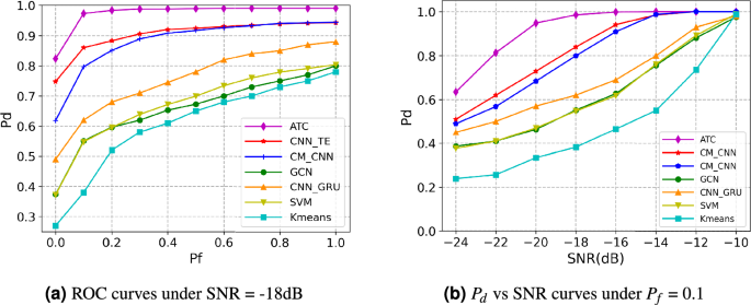

  

  Detection performance of different CSS methods under the AWGN channel.

• Under the Fading Channel: Figure 4a illustrates the ROC performance, revealing that the $\text {ATC}$ model achieved a higher AUC than the best baseline, $\text {CNN-TE}$, with an improvement of 0.1058. The result confirms the necessity of the proposed multi-branch parallel fusion strategy. The critical performance gain over the CNN-TE architecture is two-fold: it validates the superiority of parallel feature preservation over the serial transformation, and it highlights that ATC’s inclusion of the GAT branch provides the crucial spatial structure that CNN-TE lacks. Furthermore, these results in Fig. 4a emphasize the effectiveness of the CM statistic, utilized in ATC and CM-CNN, in enhancing PU detection under dynamic wireless conditions, particularly in fading channels. Figure 4b shows that the ATC model consistently achieves the highest detection probability ($P_d$) across all SNR levels. For example, at $-18 dB$, ATC achieves a $P_d$ of 84.18%, surpassing CNN-TE (66.3%), CM-CNN (63.50%), CNN-GRU, GCN, and SVM (all approximately 28%), while K-means performs the worst at 14.63%. The results indicate that models relying on energy statistics (i.e., GCN, SVM, and K-means) experience significant degradation in $P_d$ under dynamic environments such as fading channels.

Fig. 4

Detection performance of different CSS methods under the Rayleigh channel.

In this work, accuracy (Acc) is used as a general performance metric for evaluating the models’ ability to correctly detect the network states. Figure 5 presents the accuracy versus SNR on both the AWGN and Rayleigh fading channels. Consistent with the ROC and $P_d$ versus SNR results, the accuracy of all models was observed to be higher under the AWGN channel than under the Rayleigh fading channel. Furthermore, the ATC model showed the highest accuracy among the compared models under both channel types.

Fig. 5

Accuracy of different CSS methods under the AWGN and Rayleigh channels.

This study examines the effect of varying the number of SUs and PUs on detection performance. Figure 6a and b illustrate the relationship between $P_d$ and SNR for the proposed model, considering different numbers of SUs and PUs, respectively. The experiments are performed across AWGN and Rayleigh fading channels. As shown in Fig. 6a, $P_d$ improves as the number of SUs (i.e., S) increases on both channels. For instance, at SNR = $-20 dB$ under the Rayleigh fading channel, $P_d$ significantly improves with increasing S, reaching 48.13%, 68.67%, and 80.09% for S=5,10, and 15, respectively. This enhancement is attributed to the increased aggregation of PU information, leading to more accurate network state classification. Furthermore, Fig. 6a confirms that the ATC model performs better in the AWGN channel compared to the Rayleigh fading channel across different SU configurations. Notably, the number of PUs remains fixed at 2 throughout the experiments.

Fig. 6

Detection performance of the ATC model under varying the number of SUs and PUs.

Figure 6b illustrates that at low SNR values, $P_d$ improves as the number of PUs (P) increases in both AWGN and Rayleigh fading channels. Specifically, under the AWGN channel at SNR = $-24 dB$, $P_d$ for the ATC model rises from 33.6% to 72.51% as P increases from 1 to 3. This enhancement is attributed to the increased aggregate signal power from multiple PUs, facilitating the distinction between signal and noise. However, when SNR exceeds $-18 dB$, detection performance remains nearly constant regardless of P. This phenomenon occurs because, at high SNR levels, the PU signal is already sufficiently strong for accurate detection. Consequently, the number of PUs has a negligible impact, as the receiver can reliably differentiate between signal and noise.

Furthermore, the impact of the sensing period on detection performance is analyzed.

Figure 7 illustrates $P_d$ versus SNR for the proposed model under varying sensing periods in AWGN and Rayleigh fading channels. As the sensing period increases, detection probability improves across both channels. For instance, under the Rayleigh fading channel at SNR = $-20dB$, $P_d$ reaches 68.67%, 74.63%, and 78.27% for sensing periods of 200, 300, and 500 samples, respectively. This enhancement stems from the increased number of collected samples, which facilitates distinguishing PU signals from noise, thereby improving detection reliability.

Fig. 7

Pd vs SNR curves of the ATC model under varying the sensing period.

Evaluation on the real dataset

This subsection assesses the CSS models’ performance using the CSI dataset on a Wi-Fi channel across different scenarios (i.e., empty space and walking space). The dataset is constructed under the assumption of a CR network comprising a single PU equipped with one antenna and a single SU equipped with four antennas. The SU leverages its multiple antennas to collaboratively process the received signals for reliable detection of the PU’s presence.

Figure 8 illustrates the ROC curves and $P_d$ versus SNR for the models in the empty space scenario. As shown in Fig. 8a, the ATC model achieves the highest ROC among all baselines. Additionally, Fig. 8b demonstrates the superior detection probability of ATC (61.20%) compared to CNN-TE (56.72%), CM-CNN (52.80%), GCN (17%), CNN-GRU (36%), SVM (14.8%), and K-means (10%) at SNR=$-20 dB$.

Fig. 8

Detection performance of different CSS methods under the empty space.

Figure 9 presents the performance of the models in the walking space scenario, revealing a decline in detection probability compared to the empty space. This degradation stems from the increased severity of environmental dynamics caused by human movement, leading to greater signal fluctuations. As shown in Fig. 9a and b, the ATC model consistently achieves the highest detection probability in terms of both the ROC curve and $P_d$ versus SNR. Moreover, at low SNRs, models relying solely on energy statistics (i.e., GCN, SVM, and K-means) fail to detect the PU’s presence. While the CNN-GRU model captures spatial-temporal features of the received signals, it only processes local antenna-level features at the SU without leveraging inter-antenna correlations, resulting in lower detection performance compared to the ATC, CNN-TE, and CM-CNN models.

Fig. 9

Detection performance of different CSS methods under the walking space.

Figure 10 illustrates the model accuracy across the empty and walking space scenarios, demonstrating superior performance in the empty space due to reduced environmental variability. Notably, the proposed model consistently outperforms all baselines, maintaining the highest accuracy across both scenarios.

Fig. 10

Accuracy of different CSS methods under the scenarios of empty and walking spaces.

The impact of the number of sub-channels on detection performance is assessed through experiments on the proposed model. Figure 11 presents the ROC curve and $P_d$ versus SNR for the ATC model under varying sub-channel configurations ($N_{Sub-Chan}=4, 6, 8$) in both empty and walking space scenarios. The results indicate that increasing the number of sub-channels ($N_{Sub-Chan}$) enhances detection probability across both environments, likely due to the improved information extraction from the PU signals. Additionally, detection performance in the empty space remains superior to that in the walking space.

Fig. 11

Detection performance of the ATC model under varying the number of sub-channels.

Ablation study and architecture comparison

The robust performance of the proposed model stems from the synergistic combination of its specialized feature extraction branches and the parallel fusion strategy. Therefore, an ablation study is critical to validate the necessity and individual contribution of each component (GAT, CNN, Transformer encoder). To empirically justify the selection of the parallel architecture, the performance of the proposed model is directly compared against a serial architecture. We evaluate the performance of the model variants based on their ROC curves and the detection probability versus SNR on the synthetic dataset.

• Analysis of Ablation Models: This subsection analyzes the performance of the proposed model (ATC) against its ablated variants to demonstrate the necessity of the multi-branch design and the resulting superior generalization capability. Specifically, three ablated models are investigated: the model without the Transformer encoder branch (No_TE), the model without the GAT branch (No_GAT), and the model without the CM-CNN branch (No_CNN). Figures 12a(AWGN channel) and 13a(Rayleigh channel) demonstrate that the ATC model consistently achieves a superior ROC curve compared to all ablated models across both channels. This finding provides compelling evidence that the simultaneous fusion of all three distinct components is essential to maximize the model’s generalization and its discrimination capability (i.e., achieving the highest probability of detection ($P_d$) for a given probability of false alarm ($P_f$)). The performance drop observed in every ablated version confirms the non-redundant contribution of each specialized component (GAT, CNN, and Transformer encoder) to the final feature representation. Furthermore, the $P_d$ vs SNR plots of the models, reported in Figs. 12b(AWGN channel) and 13b(Rayleigh channel), consistently show that the ATC model achieves a robust probability of detection ($P_d$) across all SNR levels. This superiority is particularly pronounced in the low SNR values ($\text {i.e., } \le -20 dB$) for both channel models. Among the three ablated models, the No_CNN model exhibits a significant performance degradation. This finding underscores the critical role of the statistical features of the signal, which are inherently robust to noise. The observed performance drop resulting from the removal of any single branch confirms the necessity of the multi-branch design, proving that each component is indispensable for maintaining high detection performance under challenging channel conditions.

• Comparison of Parallel versus Serial Fusion Architecture: To provide an empirical baseline against the proposed parallel design, we construct a serial architecture model. This variant utilizes the same components (CNN, GAT, and Transformer encoder) but connects them sequentially, enforcing a predefined processing flow. The pipeline is configured as follows:

  • Initial Feature Extraction (CM-CNN): The process begins with the CM-CNN branch, utilized first to exploit the robust statistical features from the received signal (CM).

  • Spatial Relation Modeling (GAT): The resulting feature representation from the CNN output is then concatenated with the raw RSS data. This combined representation is fed into the GAT module to extract the spatial correlation structure among the SUs.

  • Temporal Dynamics Learning (Transformer encoder): Finally, the representation generated by the GAT is passed to the Transformer encoder to learn the high-level temporal dynamics of the signal.

  This sequential arrangement inherently forces the feature representation from one domain to be adapted by the next, setting the stage for a critical performance comparison with the parallel architecture where features are preserved independently until the final fusion stage. Across both Figs. 12 (AWGN channel) and 13 (Rayleigh channel), the curves corresponding to the proposed ATC model (parallel architecture) consistently surpass the performance of the serial model. This performance gap remains stable across both the $P_f$ region and the entire tested SNR range. For instance, focusing on the challenging low SNR value at SNR = $-20dB$ on the AWGN channel (Fig. 12b), the ATC model achieves $P_d$ of $94.8\%$, while the serial model reaches $P_d$ about $90.77\%$. This substantial difference demonstrates the clear superiority of the parallel fusion architecture over the serial design. This empirical superiority directly validates our theoretical argument: the serial architecture introduces information attenuation, causing the distortion or loss of valuable features (such as temporal dynamics) due to transformations in the early stages. Conversely, parallel fusion preserves the independent, pristine features from each branch, leading to a higher quality and more diverse combined representation. Crucially, this performance trend is consistent across both the AWGN channel and the more complex Rayleigh channel, demonstrating the stability and robustness of the parallel fusion design.

Fig. 12

Detection performance of ablation and serial models under the AWGN channel.

Fig. 13

Detection performance of ablation and serial models under the Rayleigh channel.

Sensitivity analysis of the RBF parameter $\rho$

As previously discussed, the parameter $\rho$ directly governs the constructed graph’s connectivity and sparsity. In this subsection, we perform a sensitivity analysis of the parameter $\rho$ on the synthetic dataset (the AWGN channel). To select the $\rho$ value, the accuracy of the proposed ATC model on the validation set is used. The selection process is essential to balance meaningful neighborhood retention against weak connection suppression.

A systematic exploration of $\rho$ values is performed, ranging from 2 to 10 (as shown in Fig. 14). This range is specifically chosen based on the mean of the pairwise distances between nodes, as it ensures the RBF kernel avoids saturation near 0 or 1. This selected range covers critical connectivity regimes, spanning from the sparse (small $\rho$) to the dense (large $\rho$).

Fig. 14

Accuracy of the ATC model when varying the parameter $\rho$ under the AWGN channel.

Figure 14 reveals a clear trend: low $\rho$ values ($\rho =2, 4$) lead to an overly sparse graph and sub-optimal performance due to insufficient spatial information for the GAT; conversely, high $\rho$ values ($\rho =8, 10$) result in an overly dense graph, introducing redundancy and noise that degrade accuracy. The model consistently achieves the robust accuracy across all tested SNR points when $\rho = 6$. This value constructs an adjacency matrix that effectively balances pruning weak, noisy connections with retaining the necessary local and mid-range relationships for efficient feature learning by the GAT. Notably, the same systematic exploration and validation technique is applied to the real-world dataset to determine its corresponding $\rho$ value.

Computational cost analysis

The computational footprint of the ATC model is illustrated in Table 4. The model utilizes 54,656 total learnable parameters (referenced from the Table 3), confirming its compact architecture and suitability for resource-constrained environments. The peak memory consumption on the NVIDIA GeForce RTX 4060 Ti during training is a manageable 4.8 GB. This low complexity and memory footprint facilitate deployment on dedicated hardware systems, enhancing the model’s practical viability for real-world applications.

Table 4 Computation cost and resource usage of the ATC Model.

The temporal efficiency of the ATC model further validates its practical significance. A rapid training cycle of the ATC model, which completed 200 epochs, takes a total of 8.77 minutes. The model demonstrates a low average inference latency, requiring only 257.5$\mu$s to process a single sample. This high throughput confirms the model’s ability to operate effectively in time-critical environments.

Discussion: interpretation of model gains

The superior performance of the proposed $\text {ATC}$ model over existing baseline methods can be primarily attributed to its multi-branch feature fusion architecture. This design intentionally integrates distinct feature extraction branches, allowing the model to capture the complex dependencies inherent in the received sensing signals at the $\text {SUs}$. Specifically, the GAT and CNN components capture neighbor-based spatial topology and localized statistical correlations, providing a robust representation of the spatial relationships. Concurrently, the Transformer encoder branch excels at modeling long-range temporal dependencies across the input sequence. This mechanism enables the subsequent classifier to leverage the synergy between the current spatial pattern and its historical temporal context. The experimental results show robust classification outcomes of the $\text {ATC}$ model, validating the hypothesis that integrating complementary statistics significantly enhances predictive power in complex environments.

Conclusion

In this study, we propose a novel CSS model tailored for CRNs involving multiple PUs. The proposed ATC model leverages DL architectures that integrate attention mechanisms, the GAT and Transformer encoder, alongside CNN, to extract rich spatial-temporal features from the received signal statistics. In particular, the GAT captures topological features among SUs based on the RSS, while CNNs are employed to capture localized statistical correlations from the CM of the received signals. Furthermore, the Transformer encoder models the temporal dynamics of the signal patterns, which reflect the activity behavior of PUs. The model’s performance is rigorously evaluated on both simulated and real-world datasets. Experimental results indicate that the proposed method can offer improved performance compared to the benchmarked CSS methods under the tested scenarios.

Despite the promising performance demonstrated by the proposed framework, the current study is subject to several limitations. A significant constraint arises from the inherent complexity of the multi-user spectrum sensing problem. Specifically, a substantial increase in the population of $\text {PUs}$ exponentially elevates the network complexity, resulting in a combinatorial explosion of possible network states. A large number of classes demands complex model architectures and extensive training data to capture all state transition dynamics. Furthermore, the evaluation of the proposed model is currently restricted to two-channel models, which may severely limit the generalization of the findings. Specifically, the model’s robustness and performance remain untested across a diverse range of realistic and challenging channel conditions, such as dynamic noise floor variations and severe fading commonly encountered in practical cognitive radio networks. In addition, although the proposed model is validated under multi-PU scenarios using synthetic datasets, the real-world dataset remains limited to the single-PU scenario due to practical data collection constraints. Future research efforts will therefore be focused on two main directions: first, to extend the framework to more diverse and realistic channel conditions (e.g., Rician fading, and shadowing effects) to validate its generalizability; and second, to address the scalability challenges associated with a large number of PUs.

References

Devroye, N., Vu, M. & Tarokh, V. Cognitive radio networks. IEEE Signal Process. Mag. 25, 12–23 (2008).
Wang, B. & Liu, K. R. Advances in cognitive radio networks: A survey. IEEE J. Select. Top. Signal Process. 5, 5–23 (2010).
Alias, D. M. et al. Cognitive radio networks: A survey. In 2016 International Conference on Wireless Communications, Signal Processing and Networking (WiSPNET) (ed. Alias, D. M.) 1981–1986 (IEEE, 2016).
Akyildiz, I. F., Lo, B. F. & Balakrishnan, R. Cooperative spectrum sensing in cognitive radio networks: A survey. Phys. Commun. 4, 40–62 (2011).
Cichoń, K., Kliks, A. & Bogucka, H. Energy-efficient cooperative spectrum sensing: A survey. IEEE Commun. Surv. Tutorials 18, 1861–1886 (2016).
Thilina, K. M., Choi, K. W., Saquib, N. & Hossain, E. Machine learning techniques for cooperative spectrum sensing in cognitive radio networks. IEEE J. Sel. Areas Commun. 31, 2209–2221 (2013).
Janu, D., Singh, K. & Kumar, S. Machine learning for cooperative spectrum sensing and sharing: A survey. Trans. Emerg. Telecommun. Technol. 33, e4352 (2022).
Somula, L. R. & Meena, M. K-nearest neighbour (knn) algorithm based cooperative spectrum sensing in cognitive radio networks. In 2022 IEEE 4th International Conference on Cybernetics, Cognition and Machine Learning Applications (ICCCMLA), 1–6 xIEEE, (2022).
Parimala, V. & Devarajan, K. Modified fuzzy c-means and k-means clustering based spectrum sensing using cooperative spectrum for cognitive radio networks applications. J. Intell. Fuzzy Syst. 43, 3727–3740 (2022).
Kumar, V., Kandpal, D. C., Jain, M., Gangopadhyay, R. & Debnath, S. K-mean clustering based cooperative spectrum sensing in generalized \(k\)-\(\mu\) fading channels. In 2016 Twenty Second National Conference on Communication (NCC), 1–5, https://doi.org/10.1109/NCC.2016.7561130 Guwahati, India, (2016).
Arkwazee, M., Ilyas, M. & Jasim, A. D. Automatic spectrum sensing techniques using support vector machine in cognitive radio network. In 2022 Second International Conference on Advances in Electrical, Computing, Communication and Sustainable Technologies (ICAECT), 1–6 IEEE, (2022).
Xu, M. et al. Cooperative spectrum sensing based on multi-features combination network in cognitive radio network. Entropy 24, 129 (2022).
Cai, L., Cao, K., Wu, Y. & Zhou, Y. Spectrum sensing based on spectrogram-aware cnn for cognitive radio network. IEEE Wirel. Commun. Lett. 11, 2135–2139 (2022).
Liu, C., Liu, X. & Liang, Y.-C. Deep cnn for spectrum sensing in cognitive radio. In 2019 IEEE International Conference on Communications (ICC), 1–6 (2019).
Liu, C., Wang, J., Liu, X. & Liang, Y.-C. Deep cm-cnn for spectrum sensing in cognitive radio. IEEE J. Sel. Areas Commun. 37, 2306–2321 (2019).
Balwani, N., Patel, D. K., Soni, B. & Lopez-Benitez, M. Long short-term memory based spectrum sensing scheme for cognitive radio. In 2019 IEEE 30th Annual International Symposium on Personal, Indoor and Mobile Radio Communications (PIMRC), 1–6 (2019).
Soni, B., Patel, D. K. & Lopez-Benitez, M. Long short-term memory based spectrum sensing scheme for cognitive radio using primary activity statistics. IEEE Access 8, 97437–97451 (2020).
Janu, D., Kumar, S. & Singh, K. A graph convolution network based adaptive cooperative spectrum sensing in cognitive radio network. IEEE Trans. Veh. Technol. 72, 2269–2279 (2022).
Veličković, P. et al. Graph attention networks. arXiv preprint arXiv:1710.10903 (2017).
Vrahatis, A. G., Lazaros, K. & Kotsiantis, S. Graph attention networks: a comprehensive review of methods and applications. Future Internet 16, 318 (2024).
Vaswani, A. et al. Attention is all you need. Advances in neural information processing systems30 (2017).
Kumar, A. et al. Analysis of spectrum sensing using deep learning algorithms: Cnns and rnns. Ain Shams Eng. J. 15, 102505 (2024).
López-Benítez, M. & Casadevall, F. Improved energy detection spectrum sensing for cognitive radio. IET Commun. 6, 785–796 (2012).
Salahdine, F., El Ghazi, H., Kaabouch, N. & Fihri, W. F. Matched filter detection with dynamic threshold for cognitive radio networks. In 2015 international conference on wireless networks and mobile communications (WINCOM), 1–6 (IEEE, 2015).
Zhang, Y. & Luo, Z. A review of research on spectrum sensing based on deep learning. Electronics 12, 4514 (2023).
Zheng, S. et al. Cooperative spectrum sensing and fusion based on tangle networks. IEEE Trans. Netw. Sci. Eng. 9, 3614–3632 (2022).
Rangaraj, N., Jothiraj, S. & Balu, S. Hybrid optimized secure cooperative spectrum sensing for cognitive radio networks. Wireless Pers. Commun. 124, 1209–1227 (2022).
Ma, J., Zhao, G. & Li, Y. Soft combination and detection for cooperative spectrum sensing in cognitive radio networks. IEEE Trans. Wireless Commun. 7, 4502–4507 (2008).
Mi, Y., Lu, G., Li, Y. & Bao, Z. A novel semi-soft decision scheme for cooperative spectrum sensing in cognitive radio networks. Sensors 19, 2522 (2019).
Malik, S. A. et al. Comparative analysis of primary transmitter detection based spectrum sensing techniques in cognitive radio systems. Aust. J. Basic Appl. Sci. 4, 4522–4531 (2010).
Sahithi, A. D., Priya, E. L. & Pratap, N. Analysis of energy detection spectrum sensing technique in cognitive radio. Int. J. Sci. Technol. Res. 9, 1772–1778 (2020).
Vijay, E. V. & Aparna, K. Rnn-birnn-lstm based spectrum sensing for proficient data transmission in cognitive radio. E-Prime-Adv. Electr. Eng. Electron. Energy 6, 100378 (2023).
Huang, W., Wang, Y., Yuan, H. & Hu, Y. Cooperative spectrum sensing algorithm based on eigenvalue and graph convolutional network. IEEE Sensors J. (2025).
Bai, W. et al. Cooperative spectrum sensing method based on channel attention and parallel cnn-lstm. Digit. Signal Process. 158, 104963 (2025).
Fang, X., Jin, M., Guo, Q. & Jiang, T. Cnn-transformer based cooperative spectrum sensing in cognitive radio networks. IEEE Wirel. Commun. Lett. (2025).
Galassi, A., Lippi, M. & Torroni, P. Attention in natural language processing. IEEE Trans. Neural Netw. Learn. Syst. 32, 4291–4308 (2020).
Guo, M.-H. et al. Attention mechanisms in computer vision: A survey. Computat. Visual Media 8, 331–368 (2022).
Choi, S. R. & Lee, M. Transformer architecture and attention mechanisms in genome data analysis: A comprehensive review. Biology 12, 1033 (2023).
Zhang, W., Wang, Y., Chen, X., Cai, Z. & Tian, Z. Spectrum transformer: An attention-based wideband spectrum detector. IEEE Trans. Wireless Commun. 23, 12343–12353 (2024).
Bai, W., Zheng, G., Xia, W., Mu, Y. & Xue, Y. Multi-user opportunistic spectrum access for cognitive radio networks based on multi-head self-attention and multi-agent deep reinforcement learning. Sensors 25, 2025 (2025).
Du, W., Wang, Y. & Qiao, Y. Recurrent spatial-temporal attention network for action recognition in videos. IEEE Trans. Image Process. 27, 1347–1360 (2017).
Hu, J., Shen, L. & Sun, G. Squeeze-and-excitation networks. In: Proc. IEEE conference on computer vision and pattern recognition, 7132–7141 (2018).
Xi, H., Guo, W., Yang, Y., Yuan, R. & Ma, H. Cross-attention mechanism-based spectrum sensing in generalized gaussian noise. Sci. Rep. 14, 23261 (2024).
Janu, D., Mushtaq, F., Mandia, S., Singh, K. & Kumar, S. Mobility-aware spectrum sensing using transformer-driven tiered structure. IEEE Commun. Lett. Massformer, (2025).
Xu, C., Jiang, B. & Su, Y. Transconvnet: Perform perceptually relevant driver’s visual attention predictions. Comput. Electr. Eng. 115, 109104 (2024).
Meneghello, F., Dal Fabbro, N., Garlisi, D., Tinnirello, I. & Rossi, M. A CSI Dataset for Wireless Human Sensing on 80 MHz Wi-Fi Channels. IEEE Commun. Magaz. (2023).
Funding
This work was supported in part by the regular research funding program (2025) of Le Quy Don Technical University under grant number 25.01.33, in part by the National Research Foundation of Korea (NRF) grant funded by the Korea government (MSIT) (No. 2022R1F1A1065516 and No. RS-2025-24523038) (O.-J.L.), and in part by the Research Fund, 2025 of The Catholic University of Korea (M-2025-B0002-00053) (O.-J.L.).
Author information
Authors and Affiliations
Contributions
D.T.L., Q.T.N., L.V.N., and O.-J.L. conceived and designed the experiments, conducted the experiments, and analyzed the results. All authors contributed to writing, reviewing, and approving the final manuscript.
Corresponding author
Ethics declarations
Competing interests
The authors declare no competing interests.
Additional information
Publisher’s note
Springer Nature remains neutral with regard to jurisdictional claims in published maps and institutional affiliations.
Rights and permissions
Open Access This article is licensed under a Creative Commons Attribution-NonCommercial-NoDerivatives 4.0 International License, which permits any non-commercial use, sharing, distribution and reproduction in any medium or format, as long as you give appropriate credit to the original author(s) and the source, provide a link to the Creative Commons licence, and indicate if you modified the licensed material. You do not have permission under this licence to share adapted material derived from this article or parts of it. The images or other third party material in this article are included in the article’s Creative Commons licence, unless indicated otherwise in a credit line to the material. If material is not included in the article’s Creative Commons licence and your intended use is not permitted by statutory regulation or exceeds the permitted use, you will need to obtain permission directly from the copyright holder. To view a copy of this licence, visit http://creativecommons.org/licenses/by-nc-nd/4.0/.
About this article
Cite this article
Lan, D.T., Ngo, Q.T., Nguyen, L.V. et al. A multi-branch network for cooperative spectrum sensing via attention-based and CNN feature fusion. Sci Rep 16, 5111 (2026). https://doi.org/10.1038/s41598-026-36031-1
Received:
Accepted:
Published:
Version of record:
DOI: https://doi.org/10.1038/s41598-026-36031-1