Assessment of ecological and landscape services in urban green spaces in South China Karst

Abstract

The assessment of urban green space (UGS) ecological and landscape services includes two aspects of ecological environment and landscape perception, which are crucial to sustainable development. Based on the three-dimensional Karst UGS environment, this study evaluates UGS ecological and landscape services using the index evaluation system with multi-dimensional attributes and the TOPSIS method. The results shows that: (1) the distribution of Karst UGS ecosystem service generally shows a “high in the east and low in the west” pattern, while the landscape perception service shows nonlinear; (2) SC has the highest weight, accounting for 20.89%; (3) the proportion of low-quality UGS was 89.63%; and (4) there is significant correlation between ecological benefit indicators. GSA has a significant correlation with the other seven indicators. This evaluation of UGS in South China Karst from ecological, residential, and social perspectives offers insights for global Karst urban management.

Introduction

Karst landforms are widely distributed across the globe, with notable regions located in eastern North America, around the Mediterranean in Europe, and centered in East Asia, particularly in southwestern China (such as Guizhou, Guangxi, Yunnan provinces)¹. These areas hold significant geological, biodiversity, and aesthetic value. The Karst areas in southern China are renowned for their unique natural formations and ecosystems, earning recognition as a UNESCO World Natural Heritage Site². It serves not only as an important scientific resource but also as a precious part of China’s natural and cultural heritage³. However, the rapid pace of urbanization⁴ is placing severe stress on the natural heritage and ecosystems of China’s southern Karst areas⁵. Karst processes have led to distinctive topographies such as stone forests, peaks, depressions, and sinkholes, yet they also result in thin soil layers with weak water retention capabilities. These geological characteristics render Karst areas ecologically sensitive, with scarce land resources, severe soil erosion, and relatively low ecosystem stability and resilience⁶. Additionally, frequent human activities have further threatened the integrity of the Karst ecosystems. As a vital component of urban ecosystems, green spaces are crucial indicators of urban ecological health. They perform multiple ecological and landscape functions, significantly contributing to improving environmental quality, regulating climate, conserving biodiversity, and providing cultural and recreational services^7,8,9. Thus, a scientific assessment of the ecological and landscape service levels of urban green spaces (UGS) in Karst areas is of great practical significance. It not only reveals the status and distribution of ecosystem services but also provides a scientific basis for sustainable regional urban development.

Under the dual pressures of a fragile ecological environment and intense human activities, the ecosystem services in Karst areas exhibit unique characteristics, reflected in provisioning, regulating, supporting, and cultural services². Research indicates that Karst ecosystems provide essential provisioning services, such as water resources, food, and energy. The subterranean rivers and groundwater in Karst regions are crucial for the daily lives of local residents and agricultural irrigation. Additionally, they serve as the primary sources of industrial water supply¹⁰. The region’s vegetation, timber, medicinal herbs, and other forest products provide essential material resources for local communities. Secondly, the regulating services in Karst areas are evident in climate regulation, water conservation (WC), soil retention, and carbon sequestration (CS) functions¹¹. The developed underground Karst systems enhance groundwater storage and regulation capabilities, effectively modulating regional water cycles and climate. Moreover, the vegetative cover aids in soil retention and CS, playing a critical role in combating rock desertification, crucial for maintaining Karst ecosystem services¹². Supporting services form the foundation for other ecological services, encompassing biodiversity, soil formation, and nutrient cycling⁵. Despite the rich biodiversity and numerous endemic species in Karst areas, ecological fragility poses significant threats to biodiversity. Additionally, unique geological conditions influence soil formation and nutrient cycling, characterized by slow soil formation, nutrient-poor conditions, and rapid water erosion due to developed Karst fissures leading to nutrient loss¹³. Lastly, cultural services are embodied in the unique natural landscapes and cultural heritage, contributing to tourism, education, research, and aesthetic appreciation. The current methods commonly used in the assessment of ecosystem services include biophysical evaluation, economic valuation, spatial assessment, and integrated evaluation^14,15. Among these, the comprehensive evaluation method stands out by selecting indicators, constructing an evaluation system, and building assessment models that can be tailored specifically for the Karst environment¹⁶. Quantitative evaluation methods mainly include: model evaluation, which uses ecological equations to assess key functions like soil retention and CS, suitable for small-scale studies¹⁷; and value equivalent methods, which assess service values based on ecosystem area, apt for large-scale studies¹⁸. Weight determination methods frequently used include the analytic hierarchy process (AHP), entropy weight method (EWM), and coefficient of variation method¹⁹. The AHP method is more subjective; the EWM reflects the degree of dispersion of the data from an objective point of view and is more influenced by the data; and the coefficient of variation method requires that the indicators are of equal importance. Each method has its advantages and limitations, with AHP-EWM combination weighting overcoming the constraints of using AHP or EWM alone²⁰, thus providing a balance of subjective and objective weighting advantages^21,22. Additionally, linear combination evaluation in multi-criteria evaluation models can determine weights, commonly applied in land suitability analysis^23,24,25.

On an urban scale, ecosystem services research is a vital branch of the field²⁶. In urban ecosystems, the concept of ecosystem services connects human societies with urban ecological systems, describing the relationship between humans and their ecological environment. UGS, embodying ecological-social-economic functions, are primary sources of urban ecosystem services, significantly enhancing residents’ quality of life and well-being²⁷. Current research on UGS ecosystem services covers topics such as carbon emission reduction²⁸ and air purification²⁹. However, despite substantial studies on UGS ecosystem services^30,31, research focused specifically on green space ecosystem services in Karst areas remains limited. The unique geological conditions in Karst areas contribute to notable regional variability in ecosystem service functions. Research indicates that Karst areas have higher water yields and soil retention rates than non-Karst areas³², giving their UGS unique geological advantages in rainwater runoff regulation, soil conservation (SC), and microclimate modulation.

The intricate terrain characteristics challenge effective assessment, optimal green space layout, and comprehensive service capacity enhancement of Karst UGS. Currently, research on Karst UGS ecosystem services often focuses on quantifying individual ecological environment service functions^33,34 or quantifying landscape cultural values alone^35,36,37. Still, comprehensive evaluations are rare and frequently disregard the human dimension. In the mountainous geographical context, the three-dimensional spatial characteristics of Karst UGS stand out, making landscape visual quality-based cultural value evaluations less reflective of local residents’ perceptions³⁸. Therefore, this study introduces indicators centered on landscape experiential perception, supplementing evaluations of visual, cultural, and aesthetic services that are difficult to directly measure³⁹, while incorporating social and economic information. In addition, SC and biodiversity conservation (BC) indicators have been incorporated into the ecosystem service assessment to describe the ecological sensitivity of Karst areas. In summary, this study constructs an AHP-EWM combined weighting TOPSIS evaluation model based on selected indicators to assess the ecological and landscape services of Karst UGS from both ecological and cultural benefits perspectives. The aim is to profoundly uncover the regional characteristics of Karst urban green areas and multidimensionally reflect their spatial information. This research provides a reference for assessing the ecological and landscape services of Karst UGS and offers insights into green space management and ecological protection in similar geomorphological areas worldwide.

Methods

Overview of the study area

Yunyan District of Guiyang City is located in Guizhou Province, China, with a geographically advantageous position at 106°29′–47′E longitude and 26°33′–41′ N latitude, as shown in Fig. 1. The district borders Wudang District to the east, Guanshanhu District to the west, and Nanming District to the south, with Baiyun District to the northwest. Covering a total area of 93.57 km², it has an average elevation of 1184 m. As of 2023, Yunyan District is home to a permanent population of 1.1535 million, renowned across Guizhou Province for having the smallest land area yet the highest population density. In terms of climate, Yunyan District experiences a typical subtropical monsoon climate, characterized by mild temperatures and abundant rainfall throughout the year. Thanks to well-executed regional planning and excellent vegetation coverage, the district showcases a harmonious coexistence between urban development and natural landscapes. As one of Guiyang’s historic urban districts, Yunyan has preserved a wealth of historical heritage throughout its urbanization process. Its Karst-dominated mountainous terrain presents unique challenges and opportunities for urban construction, shaping a city layout that adapts to the natural topography. This makes Yunyan District a quintessential example of a Karst city. Its beautiful natural environment and rich cultural heritage together contribute to the district’s distinctive charm.

Fig. 1

Map of study area.

The Karst landform, with its unique geological conditions, significantly influences the overall layout of UGS, setting it apart from typical cities and giving rise to distinctive characteristics (see Fig. 2). Firstly, due to the mountainous terrain, urban spaces develop in a three-dimensional manner. This is exemplified by the construction of pedestrian bridges and underground passages, as well as tunnels, flyovers, and elevated highways for vehicles. To save ground space, underground parking facilities are also incorporated. This design results in green spaces adopting a similarly three-dimensional configuration, such as the utilization of spaces beneath bridges and the greening of mountain slopes. Moreover, some mountainous areas remain undeveloped, coexisting with urban structures as idle green spaces, creating a unique landscape pattern of “a city within mountains and mountains within a city.” On the other hand, developed mountainous areas have been transformed into distinctive types of mountain parks. This study focuses on UGS other than idle green areas, emphasizing the uniqueness and rich diversity of UGS in Karst areas.

Fig. 2: UGS in Karst areas.

a, b Represent ancillary green spaces under overpasses, c, d represent ancillary green spaces under footbridges, and e, f represent hill greenery.

Data sources and pre-processing

The study incorporates diverse data sources, including remote sensing, meteorological, population, and survey data, as detailed below: (1) remote sensing images include: (i) GF-6 remote sensing imagery of Yunyan District, Guiyang, for 2023 was obtained from the Geovis Earth Data Cloud website (https://datacloud.geovisearth.com). The imagery, with a resolution of 2 m × 2 m, underwent preprocessing steps such as radiometric calibration, atmospheric correction, and image registration, providing high-precision geographic data for subsequent analysis. (ii) The slope data of Yunyan District is sourced from the Remote Sensing Ecology website (http://www.gisrs.cn/applists) with a resolution of 30 m × 30 m. (2) Comprehensive meteorological data include: (i) monthly temperature, precipitation, and sunshine duration for 2023, sourced from the China Meteorological Administration (https://data.cma.cn). (ii) Annual evapotranspiration data for 2020–2023, retrieved from the USGS FEWS website (https://earlywarning.usgs.gov/fews). These datasets offer a dynamic backdrop for studying the relationship between green spaces and climatic conditions. (3) Population distribution data for 2020 were acquired from the WorldPop website (https://www.worldpop.org), featuring a resolution of 100 m × 100 m. This data provides insight into the demographic characteristics of the study area. (4) Field surveys were conducted to collect questionnaires on residents’ satisfaction with nearby green spaces. Details of the questionnaire content are provided in the supplementary materials. The results are used to analyze green space usage and cultural perceptions, enriching the study’s social dimension.

In terms of data processing and analysis, the 2023 remote sensing imagery of Yunyan District was used to extract the built-up area boundaries of Yunyan District from 2020 (data sourced from the study by Li et al.⁴⁰). Combining this with the 2023 land cover classification map (dataset sourced from Li et al.⁴¹), a UGS classification and numbering system was developed using the “layer-cake” overlay mapping method. The classification process and results are illustrated in Fig. 3, with additional references to the Guiyang Public Information Platform and field surveys.

Fig. 3

UGS in the study area.

The classification results identified 135 green space patches in the study area. Specific area details for each patch are provided in Table 1.

Table 1 UGS plot area in the study area

Methodology

Figure 4 illustrates the methodological process employed in this study, which is structured into three main components: spatial analysis, evaluation model construction, and service evaluation.

Fig. 4

Research framework.

Selecting indicators and building an evaluation system is a common approach for assessing UGS⁴². Based on selection principles such as representativeness, measurability, fairness, and authority, and in conjunction with literature research⁴³, we ultimately selected eight indicators suitable for evaluating UGS in Karst cities. Given the dispersed planar layout and three-dimensional spatial characteristics of UGS in Karst areas, this study adopts three indicators from an ecological perspective to evaluate ecosystem functions, including carbon sequestration and oxygen release (CSOR), WC, air cleanness (AC), SC, and BC. Additionally, from a human-centered perspective, three supplementary indicators are selected to assess the landscape perception experience of UGS, such as green space accessibility (GSA), green view index (GVI), and resident satisfaction (RS). The detailed definitions of these indicators are provided in Table 2.

Table 2 Meaning, dimensions, and scales of evaluation indicators

The calculation method for the indicators is as follows: firstly, for every 1 ton of dry matter produced by plant growth, 1.63 tons of CO₂ are absorbed/fixed, and 1.19 tons of O₂ are released. Based on this principle and referencing relevant literature, the formula for calculating the quantitative values of the CSOR indicator is as follows⁴⁴:

$${V}_{{{CO}}_{2}}=0.4445\times {S}_{i}\times B$$

(1)

$${V}_{{O}_{2}}=1.19\times {S}_{i}\times B$$

(2)

where ${V}_{c{o}_{2}}$ represents the value of CO₂ sequestrated/fixed by plants per unit area, and ${V}_{c{o}_{2}}$ represents the value of O₂ released by plants per unit area, unit: t/hm²; ${S}_{i}$ represents the area of the ith UGS, unit: hm²; and B represents the annual net primary productivity (NPP) of plants per unit area, unit: t/(hm²·a). The value of 0.4445 is converted according to the relative molecular mass ratio of carbon to oxygen in carbon dioxide, and the carbon content is 27.27%.

Then, using the Carnegie–Ames–Stanford Approach (CASA), the NPP of Yunyan District, Guiyang City, in 2023 was estimated^45,46, yielding an average NPP of 1065.418 g C/(m²·a). The process and results are shown in Fig. 5. Therefore, in formulas (2) and (3), the value of B is set to 1065.42 g C/(m²·a), and the values of CSOR are calculated accordingly.

Fig. 5: Estimation of NPP.

a–f Represent, respectively, the vegetation index NDVI of Yunyan District, vegetation types at a 10-m resolution, monthly average temperature, precipitation, solar radiation, and NPP calculation results, all for the year 2023.

Secondly, using the water balance equation, the WC values of UGS can be estimated. The calculation formula is as follows⁴³:

$${V}_{W}=\left(P{-}{ET}{-}{R}_{i}\right)\times {S}_{i}$$

(3)

where V_W is the total amount of water source contained in the UGS, unit: m³; P is the average annual rainfall, R_i is the surface runoff, ET is the average annual evapotranspiration, all units: mm; S_i is the area of UGS, unit: m²; and i is the ith UGS in the study area.

The formula for surface runoff is calculated as follows:

$${R}_{i}=P\times {r}_{i}$$

(4)

where ${r}_{i}$ is the surface runoff coefficient, refer to the technical guide for evaluating the suitability of resources and environment carrying capacity and land and space development issued by China in 2020, as seen in Table 3.

Table 3 Coefficient of surface runoff

Based on meteorological data, the annual average evapotranspiration in the built-up area of Yunyan District in 2023 was 447.667 mm. Combining this with data from the ‘2021–2023 Guiyang Statistical Yearbook’, the annual average rainfall in Yunyan District was 1262.867 mm. According to the surface runoff coefficient, the WC capacity of each UGS was determined.

Thirdly, according to relevant literature, when the emission of pollutants exceeds the self-purification capacity of UGS, the amount of air purification service depends on the self-purification capacity of the green spaces. In the absence of significant air pollution, the pollutant emission levels are used as the basis. Based on this theory, the calculation formula for the functional value of AC is as follows⁴⁷:

$${V}_{ij}=\mathop{\sum }\limits_{j=1}^{3}Min[{A}_{j},\mathop{\sum }\limits_{i=1}^{135}{S}_{i}\times Q{S}_{ij}]$$

(5)

where ${V}_{ij}$ represents the purification amount of the ith green space absorbing the jth type of pollutant, unit: kg/hm²; ${A}_{j}$ is the emission of the jth type of air pollutant, unit: kg/hm²; ${S}_{i}$ represents the area of the ith UGS, unit: hm²; $Q{S}_{ij}$ represents the purification amount of the ith UGS per unit area for the j th type of air pollutant, unit: kg/hm²; $j$ is the type of air pollutant, $j$ = 1, 2, 3; $i$ is the UGS, $i$ = 1, 2,… 135.

Next, according to the 2023 Guiyang Statistical Yearbook and the Ecological Environment Status Bulletin, the amount of pollutants absorbed per unit area of vegetation is presented in Table 4. Based on this, the air purification capacity of UGS is calculated.

Table 4 Pollutant uptake per unit area of vegetation cover type

Fourthly, using the soil erosion force model, the SC value of UGS can be estimated⁴⁸. The calculation principle is based on the following formula:

$$SD=RKLS(1-CP)$$

(6)

In the formula, $SD$ represents the amount of SC, unit: $t/(h{m}^{2}\cdot a)$; $R$ denotes the rainfall erosivity factor, unit: $MJ\cdot mm/(h{m}^{2}\cdot h\cdot a)$; $K$ indicates the soil erodibility factor, unit: $t\cdot k{m}^{2}\cdot h/(h{m}^{2}\cdot MJ\cdot mm)$; $L$, $S$ are dimensionless slope length and slope steepness factors; $C$ represents the vegetation management factor; $P$ refers to the engineering measures factor, which takes a value of 1 for urban land⁴⁹.

The calculation method for the parameter $R,K,L,S$ and $C$ is as follows:

• A. This study directly calculates the $R$ value based on the collected monthly average precipitation data from 2023. According to Zhou et al.⁵⁰, the formula for calculating annual rainfall erosivity is as follows:

  $$R=\mathop{\sum }\limits_{i=1}^{12}-1.15527+1.792{P}_{i}$$

  (7)

  In the formula, ${P}_{i}$ represents the average precipitation for the i-th month, unit: $mm$. Based on the collected monthly average precipitation data from 2023, the calculated numerical result is 1538.681 $MJ\cdot mm/(h{m}^{2}\cdot h\cdot a)$.

• B. Using the Erosion Productivity Impact Calculator model, combined with the modified soil erodibility factor calculation formula based on China’s soil characteristics, $K$ the value can be calculated⁵¹. The calculation formula is as follows:

  $$\begin{array}{l}K=0.1317\left\{0.2+0.3\exp \left[-0.0256{S}_{d}\left(1-\displaystyle\frac{{S}_{i}}{100}\right)\right]\right\}\times {\left[\displaystyle\frac{{S}_{i}}{{C}_{l}+{S}_{i}}\right]}^{0.3}\\ \qquad\times \left[1-\displaystyle\frac{0.25TOC}{TOC+\exp (3.72-2.95TOC)}\right]\times \left[1-\displaystyle\frac{0.7S{N}_{i}}{S{N}_{i}+\exp (-5.51+22.9S{N}_{i})}\right]\end{array}$$

  (8)
  $$SN=1-\frac{{S}_{d}}{100}$$

  (9)

  In the formula, $K$ is the soil erodibility factor is, unit: $(t\cdot h{m}^{2}\cdot h)/(h{m}^{2}\cdot MJ\cdot mm)$. ${S}_{d},{S}_{i},{C}_{l}$, and $TOC$ represent the percentage content (%) of sand (0.05–2 mm), silt (0.002–0.05 mm), clay (<0.002 mm), and organic carbon according to the U.S. soil particle size classification standard, respectively.

• C. Research has shown that using the slope length formula by Fu et al.⁵² to calculate the slope length factor results in higher accuracy for the slope factor in Southwest China⁵³. Therefore, in this study, the slope length factor was calculated based on slope data obtained from the Remote Sensing Ecology official website (seen in Fig. 6) and the relevant formula, as detailed below:

  $$L={\left(\frac{l}{22.13}\right)}^{m}$$

  (10)

  Fig. 6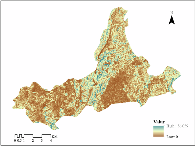

  

  The slope distribution of Yunyan District.

  In the formula, $L$ is the slope length factor; $l$ is the slope length; and $m$ is the slope length exponent, a dimensionless constant.

• D. In addition, based on their research, Liu et al.⁵⁴ proposed a modified formula for calculating the slope factor, as detailed below:

  $$S=\left(\begin{array}{cc}10.8\,\sin \theta +0.03 & \theta \,\le\, 5^{\circ} \\ 16.8\,\sin \theta -0.50 & 5^{\circ} \,<\, \theta \,\le\, 10^{\circ} \\ 20.204\,\sin \theta -1.2404 & 10^{\circ} \,<\, \theta \,\le\, 25^{\circ} \\ 29.585\,\sin \theta -5.6079 & \theta \,>\, 25^{\circ} \end{array}\right)$$

  (11)

  In the formula, $S$ is the slope factor, $\theta$ represents the slope value.

  According to the relevant literature⁵⁵, the slope length exponent and slope values applicable to the southwestern region are shown in Table 5.

  Table 5 Slope value and corresponding slope length index

• E. The formula for calculating the vegetation management factor is as follows⁵⁶:

  $$C=\left(\begin{array}{c}1\\ 0.6508-0.3436\times {\log }_{10}F\\ 0\end{array}\begin{array}{c}F=0\\ 0 \,<\, F\,\le\, 78.3 \% \\ F \,>\, 78.3 \% \end{array}\right)$$

  (12)
  $$F=\frac{NDVI-NDV{I}_{\min }}{NDV{I}_{\max }-NDV{I}_{\min }}$$

  (13)

In the formula, $F$ represents vegetation cover; $NDVI$ represents the normalized vegetation index. Given that the values of $NDV{I}_{\max }$ and $NDV{I}_{\min }$ are 0.321 and 0.226, respectively, the numerical results for $F$ and $C$ can be calculated according to the formula.

Fifthly, according to the study by Liu et al.⁴⁸, the formula for calculating biodiversity is as follows:

$${S}_{bio}=NPP\times NDVI\times SHDI\times {H}_{per}$$

(14)

In the formula, ${S}_{bio}$ represents the value of the BC index; $SHDI$ is the Shannon diversity index of green patches; ${H}_{per}$ is the habitat proportion index, which indicates the proportion of natural habitats (such as forests and grasslands) within green patches. In UGS, the ${H}_{per}$ index can be considered as 1. The Shannon diversity index of green patches can be calculated using the moving window method in Fragstats 4.2 software, as shown in Fig. 7. Substituting it into the formula provides the index value.

Fig. 7

Shannon diversity calculation for the moving window method.

Sixthly, the population-weighted green space exposure model analyzes the spatial interaction between green space distribution and population distribution from a supply-demand perspective. It assigns higher weights to green spaces located in areas with larger residential populations to assess the inequity of residents’ access to green spaces¹⁷, embodying a people-centered approach. The formula for calculating the GSA indicator in related studies is as follows, and the calculation process of GSA is illustrated in Fig. 8.

$$G{E}^{b}=\frac{{\sum }_{i=1}^{N}{P}_{i}\times {G}_{i}^{b}}{{\sum }_{i=1}^{N}{P}_{i}}$$

(15)

where ${P}_{i}$ represents the population of the $i$ th grid, ${G}_{i}^{b}$ represents the green space coverage of the ith grid for different buffer sizes, and $N$ represents the total number of grids in a given range.

Fig. 8: The GSA calculation process.

The GSA calculation process is depicted in the diagram. a The population distribution map of Yunyan’s built-up area in 2020, b the creation of a grid network, c the incorporation of green space patches, and d the GSA calculation.

Seventhly, using ArcGIS, random sampling points were generated along streets within the study area. At each point, street view images were captured in six horizontal directions and three vertical angles. Python was employed to analyze the hue of these images in HSV mode to calculate the GVI⁵⁷. The formula and its underlying principles are as follows:

$$GVI=\frac{{\sum }_{i=1}^{6}{\sum }_{j=1}^{3}{A}_{g\_ij}}{{\sum }_{i=1}^{6}{\sum }_{j=1}^{3}{A}_{t\_ij}}\times 100 \%$$

(16)

where $GVI$ represents the green visibility value of the sampling point, ${A}_{g\_ij}$ represents the number of green pixels in a single image, ${A}_{t\_ij}$ represents the total number of pixels in a single image, $i$ represents the capturing direction of the sampling point, and $j$ represents the capturing viewing angle of the sampling point.

The schematic diagram of the method and some green identification images are shown in Figs. 9 and 10, respectively.

Fig. 9

Collection of street view images.

Fig. 10

Identification of GVI.

Finally, a questionnaire was designed to assess residents’ overall satisfaction with green spaces, using a 5-point Likert scale⁵⁸, where 1 indicates “very dissatisfied” and 5 indicates “very satisfied.”, as seen in the supplementary file. The questionnaire consisted of three sections: basic demographic information, convenience of green space use, and overall perception of cultural ambiance. According to the seventh census officially published by Guiyang City, survey samples were selected using the quota sampling method to ensure that the demographic characteristics matched the overall distribution of residents in the study area. Specifically, 66.67% of the residents were between the ages of 18 and 55, while residents aged 0-18 and those aged 55 and above each accounted for 16.67%. In total, 523 valid questionnaires were obtained.

The detailed calculation results of the above indicators can be found in the “Results” section.

Based on data-driven calculations, an evaluation model is constructed using the combined weighting TOPSIS method to comprehensively assess the ecological landscape service levels of UGS. This method integrates the advantages of both subjective and objective weighting approaches and evaluates UGS quality through a relative closeness index—the closer the value is to 1, the higher the quality. The calculation process consists of two main steps: determining the weights and constructing the evaluation model.

Weight determination

The weights of each factor are calculated using the AHP and the EWM, denoted as $({\alpha }_{1},{\alpha }_{2},\cdots ,{\alpha }_{8})$ and $({\beta }_{1},{\beta }_{2},\cdots ,{\beta }_{8})$, respectively.

AHP is a method of expert scoring to determine subjective weights, and the steps are as follows: first, construct a hierarchical structure model, as seen in Fig. 11 and Supplementary Table 1. Secondly, use formula 17 to construct a judgment matrix, and then sort each layer (Supplementary Table 2) and test for consistency using formulas 18–19. Finally, the weights are determined by using formula 20 for total sorting and checking for consistency. In this study, we invited 10 experts to compare the importance of the two indicators and assign them a score (Supplementary Tables 3–5), and the identities and specific details of the 10 experts are presented in the supplementary file.

$${\rm{A}}=\left[\begin{array}{cccc}{a}_{11} & {a}_{12} & ... & {a}_{1m}\\ {a}_{12} & {a}_{22} & ... & {a}_{2m}\\ \vdots & \vdots & \ddots & \vdots \\ {a}_{m1} & {a}_{m2} & \cdots & {a}_{{mm}}\end{array}\right]$$

(17)

Where, ${a}_{ij}$ is the comparison result of the relative importance of the $i$ evaluation object and the $j$ evaluation object, and there are $m$ evaluation objects in total.

$$CR=\frac{CI}{RI}$$

(18)

$$CI=\frac{{\lambda }_{\max }-n}{n-1}$$

(19)

Fig. 11

Hierarchical model.

In the formula, $CR$ stands for the consistency ratio, $CI$ is the consistency index, ${\lambda }_{\max }$ is the maximum eigenvalue of the comparison matrix, and $n$ is the order of the matrix. When the $CR$ is less than 0.1, consistency is satisfied.

$$CR=\frac{CI}{RI}=\frac{\sum {a}_{i}C{I}_{i}}{\sum {a}_{i}R{I}_{i}}=\frac{{a}_{1}C{I}_{1}+{a}_{2}C{I}_{2}+\mathrm{..}.+{a}_{m}C{I}_{m}}{{a}_{1}R{I}_{1}+{a}_{2}R{I}_{2}+\mathrm{..}.+{a}_{m}R{I}_{m}}$$

(20)

The EWM determines the objective weights as follows: first, normalize the data using formula 21, and then use formula 22 to calculate the ratio of each indicator under the scheme. Then use formulas 23–24 to calculate the information entropy of each indicator and determine the objective weight of each indicator. Finally, the composite score is calculated using formula 25.

Suppose there are $m$ indicators: ${X}_{1},{X}_{2},\mathrm{..}.,{X}_{m}$, where ${X}_{i}=\{{x}_{1},{x}_{2},\mathrm{..}.,{x}_{n}\}$. Each indicator is subjected to positive normalization using the following calculation formula to obtain ${Y}_{1},{Y}_{2},\mathrm{..}.,{Y}_{m}$.

$${Y}_{ij}=\frac{{X}_{ij}-\,\min ({X}_{i})}{\max ({X}_{i})-\,\min ({X}_{i})}$$

(21)

$${P}_{ij}=\frac{{Y}_{ij}}{{\sum }_{j=1}^{m}{Y}_{ij}}$$

(22)

$${e}_{j}=-\,{\mathrm{ln}}{(n)}^{-1}\mathop{\sum }\limits_{i=1}^{m}{p}_{ij}{\mathrm{ln}}\,{p}_{ij}$$

(23)

In the formula, if ${p}_{ij}=0$, define ${e}_{j}=0$. The information entropy for each indicator is calculated as ${e}_{1},{e}_{2},\mathrm{..}.,{e}_{m}$。

$${\beta }_{j}=\frac{1-{e}_{j}}{{\sum }_{j=1}^{n}(1-{e}_{j})}$$

(24)

In the formula, ${\beta }_{j}$ represents the objective weight, and ${e}_{j}$ represents the information entropy.

$$S=\mathop{\sum }\limits_{j=1}^{m}{\beta }_{j}{x}_{ij}$$

(25)

In the formula, $S$ represents the comprehensive score of the quality evaluation, and ${\beta }_{j}$ represents the weight corresponding to the j-th indicator.

A target function is then established with the objective of minimizing the deviation of the combined indicator weights. By solving for the optimal linear combination coefficients, the comprehensive weights, denoted as $({\omega }_{1},{\omega }_{2},\cdots ,{\omega }_{6})$, are obtained. The calculated formula is as follows:

$${\omega }_{i}=\frac{{\sqrt{{\alpha }_{i}\beta }}_{i}}{\mathop{\sum }\nolimits_{i=1}^{n}\sqrt{{\alpha }_{i}{\beta }_{i}}}(i=1,2,\cdots ,8)$$

(26)

Evaluation model construction

The TOPSIS method is used to evaluate the quality of schemes by calculating the weighted Euclidean distances between each scheme and the positive and negative ideal solutions, thereby defining a similarity index. The evaluation process includes the following steps:

Standardizing the raw data to construct a standardized matrix Y.

$${Y}_{ij}=\frac{({X}_{ij}-{X}_{j\min })}{({X}_{j\max }-{X}_{j\min })}$$

(27)

$${Y}_{ij}=\frac{({X}_{j\min }-{X}_{ij})}{({X}_{j\max }-{X}_{j\min })}$$

(28)

Selecting indicator weights $\omega$ to create a weighted normalized matrix.

$$Z=Y\times \omega$$

(29)

Determining the positive ideal solution ${Z}^{+}$ and the negative ideal solution ${Z}^{-}$.

$${Z}^{+}=\{\max {Z}_{ij}|{\rm{j}}=1,2,\cdots ,{\rm{n}}\}=\{{Z}_{1}^{+},{Z}_{2}^{+},\cdots ,{Z}_{n}^{+}\}$$

(30)

$${Z}^{-}=\{\min {Z}_{ij}|j=1,2,\cdots ,n\}=\{{Z}_{1}^{-},{Z}_{2}^{-},\cdots ,{Z}_{n}^{-}\}$$

(31)

Calculating the distances between the evaluation objects and the ideal solutions.

$${D}_{i}^{+}=\sqrt{\mathop{\sum }\limits_{j=1}^{n}{({Z}_{ij}-{Z}_{j}^{+})}^{2}}$$

(32)

$${D}_{i}^{-}=\sqrt{\mathop{\sum }\limits_{j=1}^{n}{({Z}_{ij}-{Z}_{j}^{-})}^{2}}$$

(33)

Computing the relative closeness index ${C}_{i}$ of each evaluation object to the positive ideal solution.

$${C}_{i}=\frac{{D}_{i}^{-}}{{D}_{i}^{+}+{D}_{i}^{-}}$$

(34)

${C}_{i}$ represents the comprehensive service level of UGS, with values ranging from 0 to 1. Higher ${C}_{i}$ values indicate higher quality grades and better overall service.

The scores and corresponding quality grades are listed in Table 6. Details on weight determination and evaluation results can be found in “Results” and the analysis section.

Table 6 UGS quality grade score evaluation standard

Results

Spatial differentiation characteristics of UGS services

Figure 12 provides a description of the indicator calculation results. The findings indicate that: (1) UGS089 exhibits the best capacity of CSOR, achieving the highest CSOR values, while UGS039 performs the worst. (2) UGS089 again ranks the highest in capacity of WC, while UGS039 is the lowest. (3) UGS128 performs best in SDA, while UGS039 is the weakest; UGS089 ranks highest in nitrogen oxide absorption (NOA), while UGS039 is the lowest. UGS089 is the most effective in DR, whereas UGS046 performs the worst. (4) The strongest capacity of SC is found in UGS127, while the weakest is in UGS057; (5) UGS133 has the best capacity of BC, whereas UGS009 has the weakest capacity; (6) UGS089 has the highest value of GSA, while UGS013 has the lowest. (7) UGS115 achieves the highest overall GVI, while UGS090 scores the lowest. (8) RS with the green spaces in Yunyan District ranges from “slightly dissatisfied” to “very satisfied”. Approximately 86.67% of residents report being “moderately satisfied” or “fairly satisfied.”

Fig. 12

Numerical results of indicator calculation.

At the same time, we compared the differences in the average values of ecosystem services between two specific types of green spaces in the Karst areas: sub-bridge green space and mountain park, as seen in Fig. 13. The sub-bridge green space include UGS020, UGS062, UGS084, and UGS097, while the mountain park include UGS082, UGS102, UGS104, and UGS127. The results show that (1) the abilities related to CS, SDA, NOA, DR, and SC are superior in mountain park compared to sub-bridge green space; (2) whereas the abilities related to OR, BC, GSA, GVI, and RS are superior in sub-bridge green space compared to mountain park. The results indicate that the mountainous park excels in providing ecosystem services, while the sub-bridge green space stands out in delivering landscape perception services.

Fig. 13

Comparison of the averages of eight services between sub-bridge green spaces and mountain parks.

Kernel density analysis is a method used to calculate the density distribution of point features. The closer a location is to the center point, the higher the density value obtained; conversely, the further it is, the lower the density value⁵⁹. Using kernel density analysis, Fig. 14 illustrates the spatial distribution characteristics of UGS services in Yunyan District. Darker colors on the map indicate higher indicator values, representing better service levels. The spatial distribution results reveal that in Guiyang’s Yunyan District: (1) Ecosystem services such as CSOR, WC, AC, SC and BC generally show higher levels in the eastern part of the district and lower levels in the west. (2) GSA, GVI, and RS exhibit nonlinear distribution patterns. Specifically, GSA is relatively high in the central areas of the district but lower at the edges. GVI and RS demonstrate similar distribution trends, displaying a certain degree of regularity across the district.

Fig. 14: Spatial distribution of UGS services.

The darker the color, the higher the value.

The ecological benefit indicators assess the ecological functional value of UGS from a single dimension, with their values directly reflecting the quality of ecosystem services. The results show that UGS089 performs optimally in functions such as CSOR, WC, and NOA with DR, providing the highest level of ecosystem services, while UGS039 performs the worst, with the weakest service capabilities. Similarly, UGS127, UGS128, and UGS133 show optimal ecological functions in SDA, SC, and BC, respectively. Furthermore, the quantification results for SC indicate that the overall values across the study area are relatively low, suggesting a weak soil retention capacity of the UGS.

The humanistic benefit indicators evaluate the landscape service level of UGS from two-dimensional and three-dimensional perspectives. GSA highlights the distribution of densely populated areas—higher values indicate greater population density, better economic conditions, and higher equity in accessing green spaces. Both GVI and RS reflect the landscape perception services of UGS from a three-dimensional perspective. According to Japanese researchers, a GVI range of 0.15 to 0.25 is most beneficial for mental and physical health; when the GVI exceeds 0.25, the comfort level of residents reaches its peak⁶⁰. The study results show that the UGS of 31 fall within the optimal health range, with an additional 5 providing maximum comfort for residents. The RS indicator results suggest that RS with UGS is higher in the western and central parts of the study area.

Evaluation system for UGS services

Based on the AHP theory, we constructed an indicator evaluation system. The primary indicators include ecological benefits (B1) and humanistic benefits (B2), while the secondary indicators cover eight service evaluation metrics (C11–C15 and C21–C23). Using the scores provided by ten experts, corresponding weights were assigned to each indicator. The results, shown in Table 7, were finalized as a weight set $\alpha$. Subsequently, based on the EWM theory, the values of the eight evaluation metrics were normalized to achieve dimensionless data. The entropy method was then employed to further determine the weights, as presented in Table 8, and the final weights were recorded as set $\beta$. Finally, combined weights were calculated using Formula (17) and are denoted as $\omega$, with the results illustrated in Fig. 15.

Table 7 Determination of AHP weights

Table 8 Determination of EWM weights

Fig. 15

Distribution of indicator weights.

The combined weight results indicate that SC has the highest weight proportion (20.89%), followed by GSA (16.45%) and RS (8.05%), while GVI has the lowest proportion (2.42%). This suggests that the relative importance of the six evaluation indicators in influencing the quality of UGS in Karst areas can be ranked as: SC > GSA > RS > CSOR > AC > WC > BC > GVI.

The weighting reveals the key factors affecting green space quality. SC is the most important indicator for assessing the geological conditions of Karst areas. Studies show that while the overall terrain is relatively flat, green patches in steeper terrains have better soil retention capabilities. This aligns with the characteristic of thin topsoil in karst cities, highlighting the vulnerability and sensitivity of the Karst UGS ecosystem. Beyond two-dimensional layout information, GSA also reflects the landscape perception services of Karst UGS from social and economic dimensions. Kernel density analysis results indicate that the eastern region has better population and economic conditions compared to the western region, with higher green space equity. Moreover, RS and GVI reflect the landscape perception services of UGS from a three-dimensional perspective. However, the lower weight and correlation of GVI suggest that its importance in the construction of Karst UGS is relatively low⁶¹.

Using the TOPSIS evaluation method based on combined weighting, an evaluation system was established to calculate the relative closeness and assess the quality levels of UGS.

Results of the assessment of UGS ecological and landscape services

The relative closeness is the final calculation result in the integrated weighting TOPSIS evaluation system. A higher value indicates better UGS quality and higher overall service levels. The calculation results show that the majority of UGS falls within the range of [0, 0.2), with a total of 68, indicating that most UGS in Karst cities are of relatively low quality. The remaining UGS are categorized as follows: 53 with medium-low quality, 11 with medium quality, 2 with medium-high quality, and 1 with high quality. Figure 16 provides a detailed depiction of the quality grade distribution of UGS in Yunyan District.

Fig. 16: Assessment results of green space quality in the study area.

A darker color means lower quality.

Overall, the quality of UGS in Karst areas is predominantly concentrated in the medium-low category (including both low and medium-low quality levels), accounting for a significant 89.63%. In contrast, UGS with medium-high quality (including both medium-high and high-quality levels) represent only 2.22%. These findings indicate that the overall ecological and landscape service levels of UGS in Karst areas are relatively low. The capacity of ecosystem services is limited, and there is considerable room for improvement in landscape perception and experiential services, highlighting significant potential for enhancement.

Correlation among evaluation indicators

Figure 17 illustrates the correlations among eight indicators. The results reveal the following: (1) strong correlations are observed among CSOR, WC, AC, SC, and BC, with significance at p ≤ 0.01. (2) Except for SC, GSA has a highly significant correlation with CSOR, WC, AC, and BC indicators, with p ≤ 0.01, and a significant correlation with SC, with p ≤ 0.05. (3) GVI has a significant correlation with CSOR, WC, and SDA, and NOA within AC, with p ≤ 0.05, but is not correlated with other indicators. (4) RS is not correlated with any of the indicators, and it is particularly uncorrelated with SC. These results indicate varying degrees of interdependence among the indicators. Among them, GSA, as a socio-economic evaluation metric, is correlated with both regional ecological conditions and residents’ perceptions⁶². The GVI objectively measures the three-dimensional greening degree of green spaces in Karst cities, providing a basis for maintaining residents’ physical and mental health⁶³, and the results of the RS index are more subjective, and compared to the other six indicators, both have weaker correlations with the various indicators.

Fig. 17

The correlation analysis of each indicator’s data.

Discussion

In the mountainous Karst areas, urban construction is generally more costly, time-consuming, and labor-intensive compared to other areas. Developing cities is significantly more challenging than creating green spaces, leading to a distinctive pattern of coexistence between UGS and mountains. Consequently, the spatial arrangement of green spaces in cities located in Karst areas is characterized by fragmentation, small sizes, and poor connectivity^64,65. To comprehensively and specifically assess the ecological and landscape services of UGS in Karst cities, we developed an evaluation model based on an indicator evaluation system, employing methods such as remote sensing image interpretation, GIS spatial analysis, model estimation, and surveys. This aims to uncover the unique aspects of UGS in Karst areas from multiple dimensions. However, the model estimation method, which quantifies indicators, has limitations due to the lack of specific empirical data. Given the limited real-time monitoring data in the study area, this method is currently the most suitable for quantification, although strengthening data monitoring to provide robust support is necessary in the future. In terms of indicator selection, SC and GSA are concentrated representations of the topographic conditions of Karst UGS, and thus are assigned significant weight. Additionally, comparing distinctive types of green spaces—such as sub-bridge green space and mountain park—further highlights the unique ecological and landscape services of Karst UGS. The assessment results indicate that low-quality UGS accounts for 89.63% in Karst areas, with low ecological and landscape service levels, highlighting a need to optimize green spaces to enhance overall service levels.

Further analysis shows that the ecosystem service level of Karst UGS surpasses the average levels found in cities like Beijing, Guangzhou, and Hangzhou^66,67, although there is significant room for improvement in landscape perception services. To effectively enhance the quality of UGS in Karst areas, this study proposes recommendations and strategies in three areas: spatial layout, planning, and social benefits. Firstly, in terms of spatial layout: (i) increase green infrastructure to expand green space patches, improving overall environmental benefits. Develop idle lands moderately, explore the potential of informal green spaces⁶⁸, and utilize modern engineering technologies such as rooftop gardens to maximize space; (ii) design and promote urban green corridors to connect and integrate potential ecological pathways⁶⁹, creating a multifunctional ecological network to enhance connectivity and reduce habitat fragmentation; and (iii) align UGS with demographic characteristics by adding centralized green nodes, matching population with green resources⁷⁰. Enhance diverse transportation facilities, like greenways and paths, to reduce spatial accessibility heterogeneity, and improve access through convenient means to overcome complex mountainous terrain. Secondly, in spatial planning: (i) incorporate ecological concepts, such as rain gardens and sponge city designs, to alleviate water shortages; (ii) create diverse plant landscapes using site-specific, minimal intervention, and tree-shrub-grass combinations to establish esthetic and eco-friendly UGS; and (iii) apply modern intelligent management technologies to quickly and conveniently access big data for smart UGS management and upgrading. Lastly, concerning social benefits: (i) enhance public participation, focus on residents’ needs, and involve them in all aspects of urban planning to improve service targeting and effectiveness; (ii) increase monitoring stations and frequency, establish a comprehensive monitoring management system, foster departmental collaboration, and provide data resources for ecological research; and (iii) control urban development intensity wisely, use advanced construction technologies and eco-friendly materials, promote renewable energy and energy-saving technologies, and minimize disruptions to fragile ecosystems to achieve a harmonious integration of green space services and cultural preservation.

This study uses Yunyan District in Guiyang City—a typical city in China’s southern Karst areas—as a case study. By integrating residents’ landscape perception experiences, it evaluates the quality of Karst UGS to gauge ecological and landscape service levels. Through a model estimation method to quantify eight service indicators, it constructs an AHP-EWM weighted TOPSIS evaluation model, systematically assessing the quality of 135 UGS and yielding the following conclusions: (1) significant differences are evident in the distribution of ecosystem services and landscape perception services of Karst UGS. Ecosystem services are higher in the east than in the west, while landscape perception exhibits nonlinear distribution; (2) SC has the greatest influence on Karst UGS quality, followed by GSA, with GVI having the least effect; (3) low to medium-quality UGS account for 89.63% in Karst areas, with 68 low-quality and 53 medium-low-quality UGS, indicating overall low comprehensive service levels. High-quality green space UGS089 provides valuable reference for improving Karst UGS quality; (4) indicator correlations reveal differences between ecological and human benefits, showing strong positive correlations among ecological benefit indicators, while GSA exhibits the strongest correlation with the other seven indicators, demonstrating a certain complexity in the linkage between ecological and human benefits. Overall, the ecological and landscape service levels of UGS in Yunyan District, Guiyang City, are low. Based on these assessment results, this study offers strategic suggestions for enhancing the ecological and landscape service levels of Karst UGS through targeted strategies in spatial layout, planning, and social benefits. Future efforts should focus on preserving the historical and cultural heritage attributes of the Karst areas, further strengthening green space planning and management, establishing a robust data monitoring system, and promoting the coordination of ecological protection and urban development, thereby providing valuable insights and references for heritage site landscape management globally.

References

Ford, D. C. & Williams, P. D. Karst Hydrogeology and Geomorphology 1–5 (John Wiley & Sons, 2013); https://doi.org/10.1002/9781118684986.
Wang, K. et al. Karst landscapes of China: patterns, ecosystem processes and services. Landsc. Ecol. 34, 2743–2763 (2019).
Waltham, T. The karst lands of southern China. Geol. Today 25, 232–238 (2009).
Hu, Y., Connor, D. S., Stuhlmacher, M., Peng, J. & Turner Ii, B. L. More urbanization, more polarization: evidence from two decades of urban expansion in China. npj Urban Sustain 4, 33 (2024).
Li, S.-L., Liu, C.-Q., Chen, J.-A. & Wang, S.-J. Karst ecosystem and environment: characteristics, evolution processes, and sustainable development. Agr. Ecosyst. Environ. 306, 107173 (2021).
Paudel, S. & States, S. L. Urban green spaces and sustainability: exploring the ecosystem services and disservices of grassy lawns versus floral meadows. Urban For. Urban Green. 84, 127932 .(2023)
Galeeva, A., Mingazova, N. & Gilmanshin, I. Sustainable urban development: urban green spaces and water bodies in the city of Kazan, Russia. Mediterr. J. Soc. Sci. 5, 356–360 (2014).
Addas, A. Optimizing urban green infrastructure using a highly detailed surface modeling approach. Discov. Sustain. https://doi.org/10.1007/s43621-024-00266-7 (2024).
Huang, Z. et al. Quantifying the spatiotemporal characteristics of multi-dimensional karst ecosystem stability with Landsat time series in southwest China. Int J. Appl Earth Obs Geoinf. 104, 102575 (2021).
Lu, Y. R. Karst water resources and geo-ecology in typical regions of China. Environ. Geol. 51, 695–699 (2007).
Pu, Z. et al. Underground karst development characteristics and their influence on exploitation of karst groundwater in Guilin City, southwestern China. Carbonates Evaporites 39, 1–11 (2024).
Xiong, K., Li, J. & Long, M. Features of soil and water loss and key issues in demonstration areas for combating Karst rocky desertification. Acta Geogr. Sin. 67, 878–888 (2012).
Yan, Y., Dai, Q., Wang, X., Jin, L. & Mei, L. Response of shallow karst fissure soil quality to secondary succession in a degraded karst area of southwestern China. Geoderma 348, 76–85 (2019).
Meraj, G., Singh, S. K., Kanga, S. & Nazrul Islam, M. Modeling on comparison of ecosystem services concepts, tools, methods and their ecological-economic implications: a review. Model Earth Syst. Environ. 8, 15–34 (2022).
Häyhä, T. & Franzese, P. Ecosystem services assessment: a review under an ecological-economic and systems perspective. Ecol. Model 289, 124–132 (2014).
Li, B. et al. Spatio-temporal assessment of urbanization impacts on ecosystem services: case study of Nanjing City, China. Ecol. Ind. 71, 416–427 (2016).
Yu, Z. et al. A simple but actionable metric for assessing inequity in resident greenspace exposure. Ecol. Indic. 153, 110423 (2023).
Costanza, R. et al. The value of the world’s ecosystem services and natural capital. Ecol. Econ. 25, 3–15 (1998).
Luo, Q., Bao, Y., Wang, Z. & Chen, X. Potential recreation service efficiency of urban remnant mountain wilderness: a case study of Yunyan District of Guiyang city, China. Ecol. Indic. 141, 109081 (2022).
Cui, Y., Wang, L. & Li, L. Application of Subjective and Objective Empowerment in Evaluation of Ideological and Political Distance Learning Online Teaching 10 (EAI, 2023).
Chen, B. & Webster, C. Eight reflections on quantitative studies of urban green space: a mapping-monitoring-modeling-management (4M) perspective. Landsc. Arch. Front 10, 66–77 (2022).
de Manuel, B. F., Mendez-Fernandez, L., Pena, L. & Ametzaga-Arregi, I. A new indicator of the effectiveness of urban green infrastructure based on ecosystem services assessment. Basic Appl. Ecol. 53, 12–25 (2021).
Yakubu, S. O., Falconer, L. & Telfer, T. C. Use of scenarios with multi-criteria evaluation to better inform the selection of aquaculture zones. Aquaculture. https://doi.org/10.1016/j.aquaculture.2024.741670 (2025).
Bakolo, C. et al. Identification of optimal locations for green space initiatives through GIS-based multi-criteria analysis and the analytical hierarchy process. Environ. Syst. Res. https://doi.org/10.1186/s40068-024-00377-0 (2024).
Masoudi, M., Aboutalebi, M., Asrari, E. & Cerdà, A. Land suitability of urban and industrial development using multi-criteria evaluation (MCE) and a new model by GIS in Fasa County, Iran. Land 12, 1898 (2023).
Costanza, R. et al. The value of the world’s ecosystem services and natural capital. Nature 387, 253–260 (1997).
Zhang, S., Adam, M. & Ghafar, N. A. How satisfaction research contributes to the optimization of urban green space design—a global perspective bibliometric analysis from 2001 to 2024. Land. https://doi.org/10.3390/land13111912 (2024).
Rhea, L., Shuster, W., Shaffer, J. & Losco, R. Data proxies for assessment of urban soil suitability to support green infrastructure. J. Soil Water Conserv. 69, 254–265 (2014).
Jim, C. & Chen, W. Assessing the ecosystem service of air pollutant removal by urban trees in Guangzhou (China). J. Environ. Manag. 88, 665–676 (2008).
Liu, O. Y. & Russo, A. Assessing the contribution of urban green spaces in green infrastructure strategy planning for urban ecosystem conditions and services. Sustain. Cities Soc. https://doi.org/10.1016/j.scs.2021.102772 (2021).
Dang, H., Li, J., Zhang, Y. M. & Zhou, Z. X. Evaluation of the equity and regional management of some urban green space ecosystem services: a case study of main urban area of Xi’an city. Forests. https://www.mdpi.com/1999-4907/12/7/813# (2021).
Han, H. Q. et al. Tradeoffs and synergies between ecosystem services: a comparison of the karst and non-karst area. J. Mt Sci. 17, 1221–1234 (2020).
Xia, Z. et al. Integrating perceptions of ecosystem services in adaptive management of country parks: a case study in peri-urban Shanghai, China. Ecosyst. Serv. 60, 101522 (2023).
Liu, L., Han, B., Tan, D., Wu, D. & Shu, C. The value of ecosystem traffic noise reduction service provided by urban green belts: a case study of Shenzhen. Land 12, 786 (2023).
Yao, X. M., Chen, Y. Y., Ou, C., Zhang, Q. Y. & Yao, X. J. Spatio-temporal evolution and ecological benefits of urban green space: takes Hefei municipal area as an example. Res. Environ. Yangtze Basin 32, 51–61 (2023).
Kaplan, H., Prahalad, V. & Kendal, D. From conservation to connection: exploring the role of nativeness in shaping people’s relationships with urban trees. Environ. Manag. 72, 1006–1018 (2023).
Ko, H. & Son, Y. Perceptions of cultural ecosystem services in urban green spaces: a case study in Gwacheon, Republic of Korea. Ecol. Indic. 91, 299–306 (2018).
Rosley, M. S. F., Harun, N. Z., Yusof, J. N. & Rahman, S. R. A. Empowering public participation in assessing the indicators of aesthetic value for historical landscape: a case study on Melaka, Malaysia. Cogent. Arts Humanit. 11, 20 (2024).
Gulickx, M. M. C., Verburg, P. H., Stoorvogel, J. J., Kok, K. & Veldkamp, A. Mapping landscape services: a case study in a multifunctional rural landscape in the Netherlands. Ecol. Indic. 24, 273–283 (2013).
Li, X. et al. Mapping global urban boundaries from the global artificial impervious area (GAIA) data. Environ. Res. Lett. 15, 094044 (2020).
Li, Z. et al. SinoLC-1: the first 1-meter resolution national-scale land-cover map of China created with the deep learning framework and open-access data. EESD 15, 4749–4780 (2023).
Jiao, X., Zhao, Z., Li, X., Wang, Z. & Zhang, Y. Advances in the blue-green space evaluation index system. Ecohydrology 16, e2527 (2023).
Yang, W. Y., Li, X. & Ye, C. D. Evaluation index system for urban green system planning. Planners 9, 71–76 (2019).
Wu, W. T., Xia, G. Y. & Bao, Z. Y. The assessment of the carbon fixation and oxygen release value of the urban green space in Hangzhou. Chin. Landsc. Arch. 32, 117–121 (2016).
Potter, C. S. et al. Terrestrial ecosystem production: a process model based on global satellite and surface data. Glob. Biogeochem. Cy 7, 811–841 (1993).
Dong, D. & Ni, J. Modeling changes of net primary productivity of karst vegetation in southwestern China using the CASA model. Acta Ecol. Sin. 31, 1855–1866 (2011).
Song, C., & OUYANG, Z. Gross ecosystem product accounting for ecological benefits assessment: a case study of Qinghai province. Acta Ecol. Sin. 40, 3207–3217 (2020).
Liu, S. et al. Comparative study on two evaluating methods of ecosystem services at city-scale. Chin. J. Eco-Agric 26, 1315–1323 (2018).
Gao, C., Ding, S., Zhu, X. & Guo, J. Soil and water conservation tillage measure factor T in the CSLE model: a method review. Sci. Soil Water Conserv. 19, 142–152 (2021).
Zhou, F. & Huang, Y. The rainfall erosivity index in Fujian province. J. Soil Water Conserv. 9, 6 (1995).
Mc Bratney, A., Santos, M. & Minasny, B. On digital soil mapping. Geoderma 117, 3–52 (2003).
Fu, S., Liu, B., Zhou, G., Sun, Z. & Zhu, X. Calculation tool of topographic factors. Sci. Soil Water Conserv 13, 105–110 (2015).
Liu, C., Zhang, Y. & Wang, P. Comparative study on the two calculation methods of grid slope length factors for mountainous earth road. Subtrop. Soil Water Conserv. 34, 1–5 (2022).
Liu, B., Song, C., Shi, Z. & Tao, H. Correction algorithm of slope factor in universal soil loss equation in earth-rocky mountain area of southwest China. Soil Water Conserv. China 8, 49–52 (2015).
Guo, B., Yang, G., Zhang, F. & Liu, C. Dynamic monitoring of soil erosion in the upper Minjiang catchment using an improved soil loss equation based on remote sensing and geographic information system. Land Degrad. Dev. 29, 521–533 (2018).
Cai, C., Ding, S., Shi‘ Z., Huang‘ L. & Zhang, G. Study of applying USLE and geographical information system IDRISI to predict soil erosion in small watershed. J. Soil Water Conserv. 14, 19–24 (2000).
Li, X. et al. Assessing street-level urban greenery using Google street view and a modified green view index. Urban Forest. Urban Green. 14, 675–685 (2015).
Weber, A. S. et al. Patient opinion of the doctor-patient relationship in a public hospital in Qatar. Saudi Med. J. 32, 293–299, (2011).
Kloog, I., Haim, A. & Portnov, B. A. Using kernel density function as an urban analysis tool: Investigating the association between nightlight exposure and the incidence of breast cancer in Haifa, Israel. Comput. Environ. Urban 33, 55–63 (2009).
Wu, L. L. Research on urban road green space design based on the green looking ratio. MA Dissertation. Shanghai Jiao Tong University https://kns.cnki.net/KCMS/detail/detail.aspx?dbname=CMFD2008&filename=2008054618.nh (2008).
Conedera, M., Del Biaggio, A., Seeland, K., Moretti, M. & Home, R. Residents’ preferences and use of urban and peri-urban green spaces in a Swiss mountainous region of the Southern Alps. Urban Forest. Urban Green. 14, 139–147 (2015).
Endalew Terefe, A. & Hou, Y. Determinants influencing the accessibility and use of urban green spaces: a review of empirical evidence. City Environ. Interact. 24, 100159 (2024).
Liu, Y. et al. Psychological influence of sky view factor and green view index on daytime thermal comfort of pedestrians in Shanghai. Urban Clim. 56, 102014 (2024).
Wei, Q., He, W., Wang, J., Zhou, X. & Yao, Y. Spatial and temporal evolutionary characteristics of landscape pattern of a typical Karst watershed based on GEE platform. J. Resour. Ecol. 14, 928–939 (2023).
Wu, B., Bao, Y., Wang, Z., Chen, X. & Wei, W. Multi-temporal evaluation and optimization of ecological network in multi-mountainous city. Ecol. Indic. https://doi.org/10.1016/j.ecolind.2022.109794 (2023).
Chang, J. et al. Assessing the ecosystem services provided by urban green spaces along urban center-edge gradients. Sci. Rep. 7, 11226 (2017).
Li, F. et al. A comparative analysis of ecosystem service valuation methods: Taking Beijing, China as a case. Ecol. Indic. 154, 110872 (2023).
Rupprecht, C. D. & Byrne, J. Informal urban greenspace: a typology and trilingual systematic review of its role for urban residents and trends in the literature. Urban Forest. Urban Green. 13, 597–611 (2014).
Cui, L., Wang, J., Sun, L. & Lv, C. Construction and optimization of green space ecological networks in urban fringe areas: a case study with the urban fringe area of Tongzhou district in Beijing. J. Clean. Prod. 276, 124266 (2020).
He, M., Wu, Y., Liu, X., Wu, B. & Fu, H. Constructing a multi-functional small urban green space network for green space equity in urban built-up areas: a case study of Harbin, China. Heliyon 9, e21671 (2023).
Xiao, X., Wei, Y. K. & Li, M. The method of measurement and applications of visible green index in Japan. Urban Plan Int. 33, 98–103 (2018).
Chinese Society of Forestry. Guidelines for Ecological Restoration Through Greening Methods of Open-pit Mines. T/CSF 02-2022 (CSF, 2022).
Acknowledgements
We are deeply grateful to the Foundation for its support, including the financial assistance of the Guizhou Provincial Science and Technology Projects (No. [2024] Youth 354), the Science and Technology Innovation Talent Team Building Project of Guizhou Province (Qiankehepingtairencai-CXTD [2023] 010), and the Guizhou Provincial Basic Research Program (Natural Science) (No. QianKeHeJiChuMS [2025] 247), as well as the financial and technical support of the National Technical Innovation Center for Karst Desertification Control and Green Development (Qiankehe Zhongyindi [2023] 05). In addition, we are also grateful for the editors’ and reviewers’ reviewing.
Author information
Authors and Affiliations
Contributions
Conceptualization: X.W. and Y.C. Methodology: X.W. Data collection and analysis: X.W., X.C., and L.Y. Writing—original draft: X.W. Writing—review and editing: X.W. and Y.S. Supervision: Y.C. Funding acquisition: Y.C. and Y.S. All authors read and approved the final manuscript.
Corresponding authors
Ethics declarations
Competing interests
The authors declare no competing interests.
Additional information
Publisher’s note Springer Nature remains neutral with regard to jurisdictional claims in published maps and institutional affiliations.
Supplementary information
Rights and permissions
Open Access This article is licensed under a Creative Commons Attribution-NonCommercial-NoDerivatives 4.0 International License, which permits any non-commercial use, sharing, distribution and reproduction in any medium or format, as long as you give appropriate credit to the original author(s) and the source, provide a link to the Creative Commons licence, and indicate if you modified the licensed material. You do not have permission under this licence to share adapted material derived from this article or parts of it. The images or other third party material in this article are included in the article’s Creative Commons licence, unless indicated otherwise in a credit line to the material. If material is not included in the article’s Creative Commons licence and your intended use is not permitted by statutory regulation or exceeds the permitted use, you will need to obtain permission directly from the copyright holder. To view a copy of this licence, visit http://creativecommons.org/licenses/by-nc-nd/4.0/.
About this article
Cite this article
Wang, X., Chen, X., Yang, L. et al. Assessment of ecological and landscape services in urban green spaces in South China Karst. npj Herit. Sci. 13, 176 (2025). https://doi.org/10.1038/s40494-025-01759-y
Received:
Accepted:
Published:
Version of record:
DOI: https://doi.org/10.1038/s40494-025-01759-y