
Abstract
Seafood, including fish, prawns and various marine products, is a critical component of global nutrition due to its high protein content, essential fatty acids, vitamins and minerals. Traditional methods for assessing seafood freshness such as sensory evaluation and microbiological analysis are labor-intensive, time-consuming and often require specialized equipment. To address these limitations, this research presents an automated freshness detection system for refrigerated fish using machine learning and evaluates the effectiveness of different packaging techniques. Six seafood varieties: Mackerel, Sardine, Prawn, Pomfret, Red Snapper and Cuttlefish were stored under refrigeration and packaged using three methods: vacuum, shrink, and normal packaging. A paper-based pH sensor integrated with Methyl Red and Bromocresol Purple was utilized as a freshness indicator. This sensor effectively monitored spoilage by capturing L*, a*, and b* color values over time. Key parameters, including protein content, lipid content, and Total Volatile Basic Nitrogen (TVB-N) levels, were measured throughout the storage period to assess changes in fish quality. These measurements were used to train a Random Forest (RF) model, aimed at accurately predicting the pH values of the samples. The model’s performance was evaluated using standard metrics such as Mean Absolute Error (MAE), Mean Squared Error (MSE), and Root Mean Squared Error (RMSE). Among the tested varieties, Pomfret and Mackerel displayed the lowest MSE values (0.004625 and 0.005034, respectively), indicating high predictive reliability. The RMSE values, representing average prediction error magnitude, were also minimal for Pomfret (0.068007) and Mackerel (0.070949). Furthermore, MAE values confirmed robust predictions, with Pomfret (0.065833) and Mackerel (0.062933) achieving the least deviation from actual measurements. The study demonstrates the effectiveness of the paper-based pH sensor as a visual indicator of spoilage, while the RF-based prediction model offers a reliable method for ensuring food safety and quality during cold-chain storage. Integrating sensor-based monitoring with advanced packaging presents a viable solution for extending the shelf life of seafood and enhancing consumer safety.
Introduction
Seafood, including fish, prawns, cuttlefish and other marine products, forms a vital part of the global diet due to its high nutritional value. Rich in high-quality proteins, vitamins, minerals and essential fatty acids such as Eicosa-Pentaenoic Acid (EPA) and Docosa-Hexaenoic Acid (DHA), seafood offers numerous health benefits. These polyunsaturated fatty acids (PUFAs) contribute to improved brain function, cardiovascular health and reduced inflammation1,2. In India, the fisheries and aquaculture sector support over 14 million livelihoods and contributes significantly to national food security and economic growth through exports.
One of the major challenges in the seafood industry is maintaining product freshness during storage and distribution. The quality and shelf life of seafood are greatly influenced by packaging methods. Conventional packaging materials provide limited protection against oxygen, which can accelerate spoilage. In contrast, vacuum packaging reduces oxygen exposure, thereby inhibiting the growth of aerobic bacteria and delaying oxidative degradation. Similarly, shrink packaging helps retain moisture and forms a tight seal, further reducing oxygen penetration. Both vacuum and shrink packaging have proven effective in extending the shelf life of perishable seafood products3.
Spoilage in seafood is typically accompanied by biochemical changes, including the release of basic nitrogenous compounds like ammonia, which increases the pH of fish tissue. This change in pH can be detected using pH-sensitive colorimetric indicators. Methyl Red (MR) changes from red to yellow and Bromocresol Purple (BCP) shifts from yellow to purple as pH rises, offering a simple, real-time visual indication of spoilage4. These indicators, when embedded in paper-based biosensors, provide a non-invasive and cost-effective method for monitoring seafood freshness directly on the product.
In addition to visual indicators, scientific techniques such as Fourier Transform Infrared (FTIR) Spectroscopy are employed to analyze the chemical composition of seafood. FTIR can detect molecular changes in proteins and lipids that occur during spoilage, offering insights into degradation pathways5. Another widely accepted metric is the Total Volatile Basic Nitrogen (TVB-N) level, which measures the concentration of nitrogenous compounds like trimethylamine, dimethylamine and ammonia byproducts of microbial and enzymatic activity during spoilage6,7.
Despite the accuracy of these analytical methods, they are often time-consuming, require specialized equipment and may not be feasible for real-time monitoring across all fish species. Recent advancements in non-destructive technologies such as spectral imaging and Nuclear Magnetic Resonance (NMR) spectroscopy have addressed some of these limitations, but broad applicability remains a challenge8.
To overcome these barriers, the seafood industry is increasingly exploring the use of Artificial Intelligence (AI) and automation. Machine Learning (ML) and Deep Learning (DL) techniques have demonstrated great potential in automating food quality assessment, reducing subjectivity and enabling real-time decision-making9,10,11,12,13. These technologies can improve accuracy and efficiency in detecting seafood freshness while minimizing manual intervention14,15,16.
The novelty of this research lies in the integration of a non-invasive, paper-based pH biosensor system with machine learning techniques to enable real-time and accurate assessment of seafood freshness under refrigerated conditions. Unlike traditional sensory and microbiological methods, this approach offers a low-cost, rapid and scalable solution by using colorimetric indicators (Methyl Red and Bromocresol Purple) and correlating their L*, a*, b* color values with spoilage progression. Furthermore, the study systematically compares the effectiveness of three different packaging methods namely normal, vacuum and shrink across six commonly consumed seafood varieties. By incorporating biochemical markers such as protein, lipid content and TVB-N levels into a random forest model to predict freshness, this work presents a comprehensive framework that enhances the monitoring of seafood quality. This multifaceted strategy positions the research as a significant advancement in the automation and accuracy of seafood quality evaluation.
Materials and methods
Fish sampling
Fresh fish samples, including Mackerel (Scomber scombrus), Sardine (Sardina pilchardus), Prawn (Metapenaeus dobsoni), Black Pomfret (Parastromateus niger), Red Snapper (Lutjanus campechanus) and Cuttlefish (Sepiida), were collected immediately after harvest from the seashore market in Royapuram, Chennai, Tamil Nadu. The samples were transported to the laboratory in an ice box to maintain freshness. Upon arrival, the fish were sliced, beheaded, filleted and washed with tap water. The cleaned samples were then divided and packed using three different packaging methods: vacuum packaging, shrink packaging and regular packaging with low-density polyethylene covers. All samples were stored under refrigeration at 4 °C.
Sensor preparation
The paper-based pH sensor was prepared using two colorimetric dyes—Methyl Red and Bromocresol Purple as shown in Fig. 1 ref.17. After preparation, the sensor was placed on the surface of each fish sample. The change in color of the paper sensor was measured using a Hunter Lab Colorimeter.

Preparation of paper based sensors.
Quality analysis
The six types of fish samples, packed using three different packaging methods, were sampled at intervals of 3 days from day 0 to day 12. The experiment was conducted in triplicate. Quality parameters were analyzed at each interval. The pH of the samples was measured using a pH meter. The color values of the paper-based sensors were measured using a HunterLab XE Color Quest and used as the primary dataset. The color attributes were expressed in terms of L*, a*, and b* values, representing Lightness, Redness, and Yellowness for positive color values, and Blackness, Greenness, and Blueness for negative color values in the dried samples.
Protein content was estimated using Lowry’s method18. Fat content was determined using a Soxhlet apparatus, with petroleum ether as the solvent. Fourier Transform Infrared (FTIR) Spectral analysis was performed using a Shimadzu Irtracer 100, which has a spectral range of 4400–500 cm⁻1.
Total Volatile Basic Nitrogen (TVB-N) levels were determined using a steam distillation method with trichloroacetic acid as the solvent. The distillate was titrated with 0.01 N Hydrochloric Acid using a Rosolic Acid indicator, with the endpoint indicated by a pale pink color. TVB-N was calculated using the formula shown in Eq. (1):
where,
V1 = Volume of standard acid consumed.
W = water content of sample (g / 100 g).
Random forest model
The parameters such as L*, a*, b*, dE, protein, TVB-N, pH and fat content were obtained using the methods described above. These measurements were recorded for the different packaging methods over a 12-day period with sampling every 3 days. The collected data was used to train a random forest regression model, a powerful machine learning technique for predicting pH values.
The methodology for pH value estimation with random forest regression follows several key steps:
-
1. Data Collection: Gather a comprehensive dataset that includes all relevant features, including color metrics (L*, a*, b*, dE), protein content, TVB-N, pH and fat.
-
2. Data Preprocessing: Clean the dataset by handling missing values and outliers, normalizing numerical variables, and encoding categorical variables appropriately to prepare the data for model training.
-
3. Dataset Splitting: The dataset was divided into two subsets: a training set and a testing set. The training set was used for model training, while the testing set was used for model evaluation.
-
4. Model Training: The random forest algorithm creates an ensemble of decision trees, where each tree is trained on a random subset of the training data with replacement. A random subset of features is considered at each split, helping reduce overfitting and improving model generalization.
-
5. Hyperparameter Tuning: The hyperparameters of the random forest algorithm, such as the number of trees, the maximum depth of the trees and the minimum number of samples required to split a node, were optimized using techniques like grid search or randomized search to improve model performance.
-
6. Model Evaluation: The model’s performance was evaluated using appropriate regression metrics, including Mean Absolute Error (MAE), Mean Squared Error (MSE) and Root Mean Squared Error (RMSE). These metrics help assess how well the model predicts the pH values compared to actual values.
-
7. Model Iteration and Updates: Based on evaluation results, the model was iteratively improved by adjusting hyperparameters and feature selection techniques to enhance prediction accuracy. Additionally, the model was continuously monitored and updated to maintain its accuracy across different fish varieties, packaging methods and storage conditions.
This methodology enables consumers, suppliers and industry professionals to harness the power of machine learning for the automatic detection of pH values in seafood samples, thereby facilitating effective freshness monitoring and quality control.
Experimental results
Development of paper-based dual sensors
Paper-based sensors using Methyl Red (MR) and Bromocresol Purple (BCP) indicators were successfully developed. As shown in Fig. 2a,b, the MR sensors exhibited a pinkish-red coloration, while the BCP sensors appeared yellow under initial conditions. These sensors are pH-sensitive: an increase or decrease in pH causes the MR sensor to change from pinkish-red to yellow, whereas the BCP sensor transitions from yellow to purple. These color transitions are illustrated clearly in Fig. 3a,b.

(a) Methyl red (MR) sensor. (b) Bromocresol purple (BCP) sensor.

(a) Change in the MR sensor. (b) Change in the BCP sensor.
Fish packaging with different packaging techniques
After cleaning and filleting, all six varieties of fish were packaged using three different methods: conventional, vacuum, and shrink packaging. Low-Density Polyethylene (LDPE) and Polypropylene (PP) pouches were used for this purpose. Figure 4a,b,c show the packaging methods implemented.

(a) Conventional packaging. (b) Vacuum packaging. (c) Shrink packaging.
Colour analysis of the sensors
pH indicators used for monitoring the freshness of food typically alter their color in response to changes in the chemical composition of food samples during storage (Listyarini et al., 2018). Similarly, the color of paper-based dual sensors prepared using Methyl Red (MR) and Bromocresol Purple (BCP) indicators shifted when placed over fish samples stored under three different packaging conditions in refrigeration. To evaluate the effectiveness of these sensors, pH buffer solutions ranging from 3 to 7, with an incremental difference of 0.1, were prepared. These solutions were used to observe the corresponding color changes.
The results are presented in a graph, where the total color difference (dE) is plotted along the y-axis and the three different packaging configurations of the fish samples are plotted along the x-axis. Figure 5 illustrates the dE values of the MR sensor across different pH ranges, while Fig. 6 displays the dE values of the BCP sensor for the same pH ranges.

dE values of MR sensor at different pH range. Mean ± SD at p < 0.05 level for triplicate data.

dE values of BCP sensor at different pH range. Mean ± SD at p < 0.05 level for triplicate data.
As the pH levels in the package headspace increase during storage, volatile gases are released into the atmosphere (Fatemeh et al., 2017). Consequently, the color of the sensors changes, indicating the freshness of each sample. The findings reveal that the total color difference is more pronounced in the pH range between 4 and 6 compared to other ranges. The data further suggest that the sensors become darker as the pH approaches a more basic state, causing the color of the indicators to change accordingly.
The color of both sensors placed over the fish samples for a period of 12 days, with observations recorded at 3-day intervals, indicated that the overall color change in the sensors for Mackerel, Sardine, Cuttlefish, and Pomfret samples was relatively higher compared to Prawn and Red Snapper.
Figure 7 presents the dE values against the pH values for the MR and BCP sensors attached to vacuum-packed Sardine and Mackerel samples stored at refrigerated temperatures. Figure 8 illustrates the dE values against the pH values for MR and BCP sensors attached to vacuum-packed Prawn and Cuttlefish samples under the same storage conditions. Similarly, Fig. 9 displays the dE values against the pH values for MR and BCP sensors linked to vacuum-packed Red Snapper and Pomfret samples kept at refrigerator temperature.

dE values of MR and BCP sensors attached with sadrine and mackerel stored at refrigerator temperature.

dE values of MR and BCP sensors attached with prawn and cuttle fish stored at refrigerator temperature.

dE values of MR and BCP sensors attached with Red snapper and Pomfret stored at refrigerator temperature.
Estimation of pH
After the death of the fish, blood circulation halts, cutting off its oxygen supply. As a result, enzymes in the muscle break down glycogen into its component molecules, producing lactic acid. This process causes a decline in the pH of the fish muscle. The production of lactic acid continues until the glycogen supply is completely exhausted. Following this stage, rigor mortis sets in, characterized by muscle stiffness, which is then gradually followed by a decrease in stiffness and an increase in pH, leading to muscle softening (Tavares et al., 2021).
Data collected and presented in Table 1 shows that on the zeroth day (immediately after harvest), the pH was approximately 7, indicating that the fish was freshly caught and retained a high level of nutritional value. Fresh fish typically have a pH range of 6.0 to 6.5, characterized by firm flesh and no foul smell. Moderately fresh fish exhibit a pH range of 6.5 to 6.8, with a softer texture and mild odor, but are still considered edible. In contrast, spoiled fish have a pH greater than 6.8, sometimes exceeding 7.5, accompanied by a slimy texture and a strong ammonia-like odor. This correlation between fish freshness and pH during cold storage was also reviewed by Abbas et al.19.
As the number of storage days increased, the pH initially decreased but then began to rise gradually. This is attributed to the emission of TVB-N, which is accompanied by the production of alkaline bacterial metabolites19.
Estimation of protein
Fish, particularly Mackerel, Sardine, and Pomfret, are well-known for their high protein content. To quantify the protein levels in fresh fish samples, Lowry’s method was employed, and the results are presented in Table 2. When the experiment was repeated at 3-day intervals, it was observed that the protein content gradually decreased over time. This decline was not abrupt but progressive. The reduction in protein levels is primarily attributed to autolysis, an intrinsic breakdown of proteins and fats caused by a series of complex enzyme reactions.
Since the samples were stored under refrigerated conditions, the rate and extent of protein degradation were significantly minimized. Shenouda et al. (1980) demonstrated that several factors contribute to protein loss in fish during refrigeration, including enzyme-mediated activity of trimethylamine oxide (TMAO), an increase in solute concentration, dehydration, the formation of ice crystals, and accretion.
Estimation of fat
Hydrolysis and oxidation are two distinct chemical reactions that occur during the processing and storage of fish, both contributing to the reduction of fat content. During lipid hydrolysis, free fatty acids are released, leading to the denaturation of proteins as their structure is compromised (Bashir et al., 2021). It was observed that the fat content decreased progressively as the storage period increased.
After being refrigerated for 12 days, the fat content in the fatty fish Mackerel and Sardine dropped from 12 to 9 g and 11 to 9 g, respectively. A similar trend was observed in the other four fish samples: Red Snapper, Cuttlefish, Pomfret and Prawn. The results are summarized in Table 3. The reduction in lipid content during refrigerated storage is primarily attributed to oxidation. This oxidative reaction generates peroxides, which accelerate the degradation of fish quality (A. Keyvan et al., 2008).
Results of random forest model
The random forest model was trained using data collected from six different varieties of fish, each packed using different packaging methods. Table 4 presents the observed values for L*, a*, b*, dE, pH, protein and fat over a period of 0 to 12 days under refrigerated conditions.
The random forest model was trained separately for each variety of fish. The decision tree generated for the Prawn variety is shown in Fig. 10. The decision tree possesses several essential characteristics that define its structure and functionality. At the root node, the initial condition is established as protein ≤ 11.775, which splits the dataset into two branches: the left branch if the condition is true, and the right branch if it is false. Intermediate nodes further refine the data subsets. For example, in the left subtree, further divisions occur based on criteria such as package ≤ 0.5. Similarly, the right subtree branches off according to parameters like TVB-N ≤ 11.32 and dE ≤ 34.73.
Decision tree from random forest for prawn.
Leaf nodes, represented as terminal boxes, indicate the final predictions of the tree. Each node in the tree displays the number of samples that reach that specific point. Additionally, the squared error at each node serves as a measure of predictive accuracy, where smaller values signify better performance.
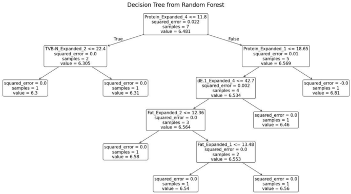
The random forest model was trained separately for each variety of fish. The decision tree generated for the fish variety Pomfret is shown in Fig. 11. This decision tree possesses several key characteristics that define its structure and functionality. At the root node, the initial condition is established as protein ≤ 14.175, which divides the dataset into two branches: the left branch if the condition is true and the right branch if it is false. Intermediate nodes further refine the data subsets. For example, in the left subtree, additional splits occur based on criteria such as TVB-N ≤ 15.035. Similarly, in the right subtree, divisions are made according to parameters like dE ≤ 28.66.
Decision tree from random forest for Pomfret.
Leaf nodes, represented as terminal boxes, indicate the final predictions of the tree. These leaf nodes mark the completion of the decision-making path, where the model assigns a prediction based on the features observed.
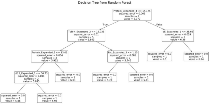
The random forest model was trained separately for each variety of fish. The decision tree generated for the fish variety Red Snapper is shown in Fig. 12. This decision tree possesses several key characteristics that define its structure and functionality. At the root node, the initial condition is established as protein ≤ 21.77, which divides the dataset into two branches: the left branch if the condition is true and the right branch if it is false. Intermediate nodes further refine the data subsets. For example, in the left subtree, additional splits occur based on criteria such as TVB-N ≤ 11.815. Leaf nodes, represented as terminal boxes, indicate the final predictions of the tree. These leaf nodes mark the end of the decision-making path, where the model makes its final prediction based on the observed features.
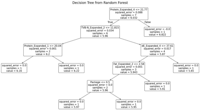
Decision tree from random forest for red snapper.
The random forest model was trained separately for each variety of fish. The decision tree generated for the fish variety Sardine is shown in Fig. 13. This decision tree possesses several key characteristics that define its structure and functionality. At the root node, the initial condition is established as fat ≤ 12.545, which divides the dataset into two branches: the left branch if the condition is true and the right branch if it is false. Intermediate nodes further refine the data subsets. For example, in the left subtree, additional splits occur based on criteria such as TVB-N ≤ 23.715. Similarly, the right subtree is divided according to parameters like TVB-N ≤ 18.08. Leaf nodes, represented as terminal boxes, indicate the final predictions of the tree. These leaf nodes mark the conclusion of decision paths, where the model outputs its final prediction based on the observed features.
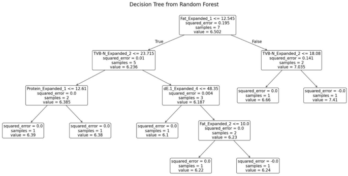
Decision tree from random forest for sardine.
The random forest model was trained separately for each variety of fish. The decision tree generated for the fish variety Mackerel is shown in Fig. 14. This decision tree possesses several key characteristics that define its structure and functionality. At the root node, the initial condition is established as protein ≤ 9.84, which divides the dataset into two branches: the left branch if the condition is true and the right branch if it is false. Intermediate nodes further refine the data subsets. For example, in the left subtree, additional splits occur based on criteria such as TVB-N ≤ 22.67. Similarly, the right subtree is divided according to parameters like dE ≤ 28.83. Leaf nodes, represented as terminal boxes, indicate the final predictions of the tree. These leaf nodes mark the end of decision paths, where the model outputs its final prediction based on the observed features.
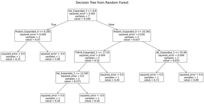
Decision tree from random forest for mackerel.
The random forest model was trained separately for each variety of fish. The decision tree generated for the fish variety Cuttlefish is shown in Fig. 15. This decision tree exhibits several key characteristics that define its structure and functionality. At the root node, the initial condition is set as TVB-N ≤ 22.23, which divides the dataset into two branches: the left branch if the condition is true and the right branch if it is false. Intermediate nodes further refine the data subsets. For example, in the left subtree, additional splits occur based on criteria such as fat ≤ 3.125. Leaf nodes, represented as terminal boxes, indicate the final predictions of the tree. These leaf nodes mark the end of decision paths, where the model outputs its final prediction based on the observed features.
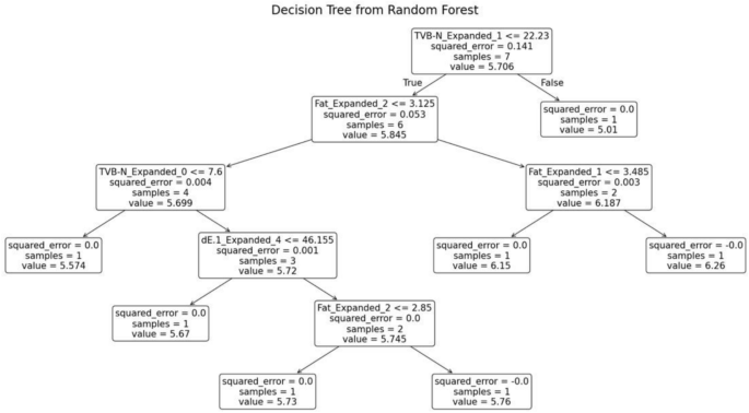
Decision tree from random forest for Cuttle fish.
The random forest model generates multiple decision trees during the training phase. When testing the model, an unknown sample is provided, and the model predicts its pH value. The performance of the random forest model is assessed using evaluation metrics such as Mean Absolute Error (MAE), Mean Squared Error (MSE), and Root Mean Squared Error (RMSE). Table 5 presents the predicted pH values alongside the corresponding evaluation metrics.
The freshness of the fish is classified into three categories namely Fresh, Moderately Fresh, and Spoiled based on the predicted pH values using the trained Random Forest model. The freshness category for each fish type on the 15th day of vacuum storage is shown in Table 6.
Conclusion
In conclusion, the paper-based dual sensors were successfully developed, and their efficiency was evaluated by comparing the color values obtained from buffer solutions with those of the sensors placed over refrigerated fish samples. The total amount of protein and fat in the fish samples stored under refrigeration for an extended period showed a gradual decline. This decrease is attributed to the refrigeration process, which, through the formation of ice crystals, inhibits the chemical reactions that typically lead to fish spoilage. As a result, the depletion of nutrients was less severe.
The rate of spoilage in vacuum packaging was found to be significantly slower compared to conventional and shrink packaging. This clearly demonstrated that vacuum packaging is the most effective method for preserving fish. After 12 days of storage, there was only about a 2% reduction in the total protein and fat content of the fish samples. Following the rigor mortis phase, the pH levels of the samples initially dipped slightly but began to rise again after a few days. After being refrigerated at 4 °C (± 3 °C) for a period of 12 days, the fish samples underwent TVB-N Estimation. The results indicated that the fish remained safe for consumption, as the level of volatile nitrogen in all six fish samples was less than 35 mgN/100 g.
Furthermore, the automation of freshness detection for refrigerated fish using a random forest model was successfully developed. The evaluation metrics Mean Absolute Error (MAE), Mean Squared Error (MSE), and Root Mean Squared Error (RMSE) demonstrated that the model accurately detected the freshness of the fish. This is particularly significant for advancing food processing automation.
Data availability
The datasets used and/or analysed during the current study available from the corresponding author on reasonable request.
References
Farooqui, A. & Farooqui, A. A. Fish oil and importance of its ingredients in human diet. Benef. Eff. Fish Oil Hum. Brain https://doi.org/10.1007/978-1-4419-0543-7_5 (2009).
Mazer, L. M., Yi, S. H. & Singh, R. H. Docosahexaenoic acid status in females of reproductive age with maple syrup urine disease. J. Inherit. Metab. Dis. 33, 121–127 (2010).
KashaniZadeh, H. et al. Rapid assessment of fish freshness for multiple supply-chain nodes using multi-mode spectroscopy and fusion-based artificial intelligence. Sensors 23(11), 5149. https://doi.org/10.3390/s23115149 (2023).
Kuswandi, B., Damayanti, F., Abdullah, A. & Heng, L. Y. Simple and low-cost on-package sticker sensor based on litmus paper for real-time monitoring of beef freshness. J. Math. Fund. Sci. https://doi.org/10.5614/j.math.fund.sci.2015.47.3.2 (2015).
Sanden, K. W. et al. The use of fourier-transform infrared spectroscopy to characterize connective tissue components in skeletal muscle of Atlantic cod (Gadus morhua L.). J. Biophoton. 12(9), e201800436 (2019).
Moosavi-Nasab, M., Khoshnoudi-Nia, S., Azimifar, Z. & Kamyab, S. Evaluation of the total volatile basic nitrogen (TVB-N) content in fish fillets using hyperspectral imaging coupled with deep learning neural network and meta-analysis. Sci. Rep. 11(1), 5094 (2021).
Tahsin, K. N., Soad, A. R., Ali, A. M. & Moury, I. J. A review on the techniques for quality assurance of fish and fish products. Int. J. Adv. Res. Sci. Eng. 4, 4190–4206 (2017).
Prabhakar, P. K., Vatsa, S., Srivastav, P. P. & Pathak, S. S. A comprehensive review on freshness of fish and assessment: Analytical methods and recent innovations. Food Res. Int. 133, 109157 (2020).
Kotteti, C., Sadiku, M. & Musa, S. Machine learning in automation. Int. J. Adv. Sci. Res. Eng. https://doi.org/10.31695/IJASRE.2018.327561 (2018).
Wang, Dakuo and Andres, Josh and Weisz, Justin D. and Oduor, Erick and Dugan, Casey. (2021). AutoDS: Towards human-centered automation of data science. Proceedings of the 2021 CHI Conference on Human Factors in Computing Systems.
Zhu, L., Spachos, P., Pensini, E., & Plataniotis, K. Deep learning and machine vision for food processing: A survey. arXiv preprint arXiv:2103.16106. (2021).
Liu, X., Liang, J., Ye, Y., Song, Z., & Zhao, J. A food package recognition and sorting system based on structured light and deep learning. arXiv preprint arXiv:2309.03704. (2023).
Rokhva, S., Teimourpour, B., & Soltani, A. H. Computer vision in the food industry: Accurate, real-time, and automatic food recognition with pretrained MobileNetV2. arXiv preprint arXiv:2405.11621. (2024).
Arachchige, U., Chandrasiri, S. & Wijenayake, A. Development of automated systems for the implementation of food processing. J. Res. Technol. Eng. 3, 2022–2030 (2022).
Chao, K., Kim, M. S. & Lu, R. Food process automation. Sens. Instrument. Food Qual. Saf. 3(1), 1932–9954 (2009).
Nedumaran, Dr. & Ritha, M. Robotics revolution: transforming the food industry through automation and innovation. SSRN Electron. J. 2, 165–170. https://doi.org/10.2139/ssrn.4758029 (2024).
Kuswandi, B. & Nurfawaidi, A. On-package dual sensors label based on pH indicators for real-time monitoring of beef freshness. Food Control 82, 91–100 (2017).
Remya, V. K., Vinitha, M. S. & Jijisha, T. S. A comparative study of nutritive value in fresh and salt dried fish. Int. J. Adv. Eng. Manag. (IJAEM) 3(3), 259 (2021).
Abbas, K. A., Mohamed, A., Jamilah, B. & Ebrahimian, M. A review on correlations between fish freshness and pH during cold storage. Am. J. Biochem. Biotechnol. 4(4), 416–421 (2008).
Author information
Authors and Affiliations
Contributions
B. Kumaravel: Conceptualization, Experimentation, Methodology, Writing A. L. Amutha: Conceptualization, Data Curation, Writing—Original Draft, Supervision. Milintha Mary T P: Experimentation, Data Curation, Writing—Original Draft. Aryan Agrawal: Data Collection, Machine Learning Model Development. Akshat Singh: Experimentation, Data Analysis, Visualization. Saran S: Experimentation, Validation, Data Interpretation. Nagamaniammai Govindarajan: Project Administration, Resources, Writing—Review & Editing. All authors have read and approved the final manuscript.
Corresponding author
Ethics declarations
Competing interests
The authors declare no competing interests.
Additional information
Publisher’s note
Springer Nature remains neutral with regard to jurisdictional claims in published maps and institutional affiliations.
Rights and permissions
Open Access This article is licensed under a Creative Commons Attribution-NonCommercial-NoDerivatives 4.0 International License, which permits any non-commercial use, sharing, distribution and reproduction in any medium or format, as long as you give appropriate credit to the original author(s) and the source, provide a link to the Creative Commons licence, and indicate if you modified the licensed material. You do not have permission under this licence to share adapted material derived from this article or parts of it. The images or other third party material in this article are included in the article’s Creative Commons licence, unless indicated otherwise in a credit line to the material. If material is not included in the article’s Creative Commons licence and your intended use is not permitted by statutory regulation or exceeds the permitted use, you will need to obtain permission directly from the copyright holder. To view a copy of this licence, visit http://creativecommons.org/licenses/by-nc-nd/4.0/.
About this article

Cite this article
Kumaravel, B., Amutha, A.L., Mary, T.P.M. et al. Automated seafood freshness detection and preservation analysis using machine learning and paper-based pH sensors. Sci Rep 15, 26051 (2025). https://doi.org/10.1038/s41598-025-08177-x
Received:
Accepted:
Published:
Version of record:
DOI: https://doi.org/10.1038/s41598-025-08177-x
