
Abstract
Sparse numerical datasets are dominant in fields such as applied mathematics, astronomy, finance, and healthcare, presenting challenges due to their high dimensionality and sparse distribution. The predominance of zero values complicates optimal feature selection, making data analysis and model performance more complex. To overcome this challenge, this study introduces a deep learning-based algorithm, Hybrid Stacked Sparse Autoencoder (HSSAE), which integrates \({\text{L}}_{1}\) and \({\text{L}}_{2}\) regularization with binary cross-entropy loss to improve feature selection efficiency, where \({\text{L}}_{1}\) regularization penalizes large weights, simplifying data representations, while \({\text{L}}_{2}\) regularization prevents overfitting by limiting the total weight size. Additionally, the dropout technique enhances the algorithm’s performance by randomly deactivating neurons during training, avoiding over-reliance on specific features. Meanwhile, batch normalization stabilizes weight distributions, reducing computational complexity and accelerating the convergence. The proposed algorithm, HSSAE, was evaluated against traditional classifiers, including Decision Tree, Random Forest, K-Nearest Neighbors, and Naïve Bayes, as well as deep learning-based models, such as Convolutional Neural Network, Long Short-Term Memory, and Stacked Sparse Autoencoder, in terms of Precision, Recall, Accuracy, F1-score, AUC, and Hamming Loss. Quantitatively, the proposed algorithm, HSSAE, was tested on two different sparse datasets, demonstrating superior performance with the highest accuracy of 89% on the health indicator dataset and 93% on the EHRs diabetes prediction dataset, respectively, and outperforming competing classifiers. The proposed algorithm, HSSAE, extracts features effectively and enhances robustness, making it well-suited for sparse data applications, particularly in healthcare, where high prediction accuracy is crucial.
Introduction
Diabetes is a chronic metabolic disorder, sometimes with autoimmune origins, whose rising prevalence is strongly shaped by environmental and genetic factors1. In 2010, approximately 285 million people worldwide were affected, a number projected to rise to 552 million by 2030, representing 6.4% of the global adult population2. Diabetes is broadly classified into three types: Type 1, Type 2, and gestational diabetes. Type 1 diabetes, an autoimmune disorder in which the pancreas fails to produce insulin, typically develops in children and young adults under 30 years of age, and insulin therapy remains the primary treatment. Type 2 diabetes, in contrast, is associated with insulin resistance, obesity, and ageing, occurring more frequently in individuals over 65 years. Unlike Type 1, Type 2 can often be predicted, prevented, or diagnosed based on family history, gender, and lifestyle factors. Gestational diabetes develops during pregnancy and may result in maternal hyperglycemia3. Early diagnosis of diabetes is critical, and technological tools play an important role in identifying clinical indicators, reducing human error, and streamlining assessments4. However, clinical datasets are often underutilized due to heterogeneity, high dimensionality, and sparsity. Sparse data is a well-recognised challenge not only in healthcare but also in recommender systems, genomics, and natural language processing (NLP). In recommender systems, matrix factorization and collaborative filtering techniques are used to address sparsity in user–item interactions5. In genomics, dimensionality reduction and regularization methods help manage high-dimensional yet sparse gene expression data6. Similarly, in NLP, word embeddings and transformer-based models mitigate sparsity in text representations7. These strategies suggest possible solutions that could be adapted to healthcare, where datasets are often both sparse and high-dimensional. Given these challenges, Machine Learning (ML), an expanding subfield of artificial intelligence, offers significant promise, as it can capture nonlinear relationships in complex datasets and automatically learn patterns without explicit programming8,9,,9.
Chang et al.10 studied a sparse dataset of health indicators for early diabetes prediction and diagnosis, utilising ML approaches, notably Decision Trees (DT), Random Forests (RF), K-Nearest Neighbours (KNN), Logistic Regression (LR), and Naive Bayes (NB). These common ML algorithms often struggle to extract significant features from sparse datasets, resulting in lower accuracy. Furthermore, driven by advances in computational power, Deep Learning (DL), a frontier approach in ML, has recently achieved remarkable success, often surpassing state-of-the-art methods across various healthcare domains11,12,13.
Despite extensive literature reviews on the use of artificial intelligence (AI) for diabetes, which include some traditional ML methods and statistical models, systematic research remains lacking, focusing on DL applications for diabetes14,15,16. For instance, Pathak et al.17 examined the prediction gap for type 2 diabetes using rigorous learning methods. However, they noted that the available data are often less precise. The majority of research publications have predominantly employed ML techniques for diabetes prediction. Although DL algorithms have been extensively applied to the prediction of various diseases, their application to type 2 diabetes remains relatively limited. Zhang et al.18 provided a non-invasive approach that uses the stacked sparse autoencoder methodology to identify diabetes mellitus in a dataset of facial images. Additionally, Kannadasan et al.19 developed a Deep Neural Network (DNN) for diabetic data classification applied to the Pima Indians’ diabetes dataset. DNN employs stacked autoencoders and SoftMax for feature extraction and classification. However, the Pima Indians’ diabetes dataset has 12% sparse data, and DNN fails to manage and support it. Their findings demonstrate that sparse data issues in diabetes prediction necessitate strong techniques. Furthermore, Alex et al.20 developed a Deep Convolutional Neural Network (CNN) for diabetes prediction, utilising data from Electronic Health Records (EHRs) for training. However, this model relies on massive, labelled datasets, making it computationally intensive and difficult to interpret. Similarly, Vivekanandan et al.21 proposed the Stacked Autoencoder for feature learning, extraction, and classification using shallow and DNN, utilising the Indian Pima dataset. However, as the data is sparse, this model struggles to extract the relevant features, resulting in lower classification accuracy. Further, García et al.22 proposed a DL approach, such as a variational autoencoder for data augmentation, a stacked autoencoder for feature extraction, and a CNN for the prediction of type 2 diabetes using the Indian Pima dataset as well. However, the limited dataset size constrained the model’s performance.
Thaiyalnayaki et al.23 used the Indian Pima dataset to predict type 2 diabetes with Multilayer Perceptrons (MLPs) and support vector machines. The MLP classifier fine-tunes the hyperparameters to minimise the loss function and optimise the model, but the model has difficulty extracting features and cannot provide adequate accuracy. This limitation is largely attributed to the small dataset, which restricts the model’s ability to generalize effectively. Also, Miotto et al.24 proposed a Stack Denoising Autoencoder (SDA) for predicting type 2 diabetes using an EHR dataset, which enables the capture of complex patterns in EHRs without the need for manual feature engineering. However, it relies solely on the frequency of the laboratory test without considering the actual test result, resulting in low predictive power for the disease. Moreover, Chetoui et al.25 developed a federated learning framework that employs Vision Transformers for diabetic retinopathy detection, enhancing accuracy while preserving data privacy. However, the model demonstrated limitations when applied to larger imbalanced datasets, such as Eyepacs, and faced challenges associated with high-dimensional sparse data, including overfitting, difficulties in feature selection, and increased computational complexity. Similarly, Lan et al.26 introduced a Higher-Dimensional Transformer (HDformer) for diabetes detection using PPG signals, achieving high performance accuracy and enhanced computational efficiency through the Time Square Attention (TSA) module. Nevertheless, the model faced challenges with real-world noise in PPG signals, limited scalability for longer signal periods, and poor generalization due to small or imbalanced datasets. Beyond these task-specific architectures, transformer-based frameworks such as Medical Bidirectional Encoder Representations from Transformers (Med-BERT), Bidirectional Encoder Representations from Transformers for Electronic Health Records (BEHRT), and Tabular Neural Attention Network (TabNet) have also been applied in broader healthcare contexts. Med-BERT and BEHRT utilize self-attention mechanisms for EHR modelling, thereby improving sequence learning and disease prediction27,28. While TabNet is utilised for structured tabular data, it demonstrates effectiveness in managing high-dimensional clinical datasets29.
These models highlight the potential for healthcare tasks; however, their performance may still be constrained by sparsity, high dimensionality, and domain adaptation challenges, encouraging further investigation into this area. Prior studies in healthcare, particularly in disease prediction using DL algorithms, have shown that these algorithms often focus on dense datasets where most values are non-zero and struggle to extract functional characteristics from sparse data collections effectively. Table 1 provides an overview of various machine learning and deep learning models, highlighting their advantages and limitations.
Healthcare datasets often contain numerous sparse values; however, removing these values can substantially reduce the dataset size, ultimately compromising predictive accuracy. Therefore, careful feature selection is essential to minimize the risk of false predictions. Therefore, the primary objective of this study is to accurately predict Type 2 diabetes using two sparse diabetes datasets with the proposed deep learning-based algorithm HSSAE. The main contributions of this study are outlined below.
-
I.
Develop an HSSAE algorithm as an advanced autoencoder-based deep learning framework for identifying key features associated with high-risk factors in diabetes prediction.
-
II.
Propose a hybrid loss function that integrates \({\text{L}}_{1}\) and \({\text{L}}_{2}\) regularization with a single parameter \(\alpha\) with binary cross-entropy loss to improve feature selection efficiency in sparse datasets.
-
III.
Gauge the performance and reliability of the proposed HSSAE algorithm using Precision, Recall, Accuracy, F1-score, AUC, and Hamming Loss as key assessment metrics.
-
IV.
Evaluate the HSSAE algorithm against traditional classifiers, including DT, RF, KNN, NB, and DL models, such as CNN, LSTM, and SSAE, demonstrating its superior accuracy on both Type 2 diabetic datasets.
The rest of the paper is organized as follows: Section “Materials and methods” describes the dataset, preprocessing techniques, and the architecture of the proposed HSSAE model. Section “Experiments and analysis” details the experimental setup, evaluation metrics, and comparative analysis with traditional ML and DL models. Section “Discussion” provides an in-depth interpretation of the results, emphasizing the proposed algorithm HSSAE strengths and areas for improvement. Finally, Section “Conclusion” summarizes the key findings, discusses the implications, and outlines potential future research directions.
Materials and methods
In the prediction of diabetes using the HSSAE algorithm, the research was conducted in three stages, as indicated in Fig. 1. Initially, the dataset was pre-processed using the Synthetic Minority Over-sampling Technique (SMOTE) in conjunction with min–max normalization. Following the pre-processing stage, the statistical analysis was performed to determine the nature of the data. Subsequently, the HSSAE algorithm was developed and trained with the pre-processed dataset. The HSSAE algorithm was employed to identify the complex patterns within the dataset, which were subsequently utilized for the prediction tasks. Finally, the performance of the algorithm, HSSAE, was evaluated using several metrics, including accuracy, precision, recall, F1 score, AUC, and Hamming loss. These metrics provided a comprehensive overview of the algorithm’s performance in diabetes prediction.

Framework of the study from data collection to evaluation.
Data acquisition, statistical analysis, and preprocessing
This study utilized the Diabetes Health Indicators Dataset (DHID), collected by the Centers for Disease Control and Prevention (CDC) via a telephone survey and available on Kaggle at “https://www.kaggle.com/datasets/alexteboul/diabetes-health-indicators-dataset”. The Health Indicator Dataset comprises 253,680 rows and 21 columns, with a sparsity of 43%, indicating that a substantial portion of the data contains zero values. Additionally, the EHRs Diabetes Prediction Dataset, accessible at “https://www.kaggle.com/code/ahmadkaif/diabetes-prediction”, was employed for diabetes prediction tasks. This dataset contains diverse patient information, including medical history, demographic data, and diabetes status, representing typical features of real-world clinical datasets. Initially, the dataset’s sparsity rate was 31%. To assess the robustness of the proposed HSSAE model under higher sparsity, we systematically increased the sparsity of selected numerical features (e.g., age, BMI, HbA1c level, and blood glucose level) by randomly setting 70% of their entries to zero, using a fixed random seed to ensure reproducibility. After this procedure, the sparsity of the selected features reached approximately 73%. The sparsity of each dataset was calculated using Eq. (1).
Statistical analysis of the sparse health indicators diabetes dataset
The dataset comprises two categories of variables: Numerical and Categorical. Numerical variables are quantitative measures such as Body Mass Index (BMI), general health, mental health, age, education level, and income, as presented in Table 2. BMI, with a mean of 28.38, high skewness (2.12), and kurtosis (10.99), highlights the presence of extreme obesity cases that are strongly linked to diabetes onset. General health, with a mean of 2.51, exhibits low skewness (0.42) and kurtosis (− 0.38), suggesting that most participants reported average health. Mental health (mean 3.18) and physical health (mean 4.24) show high variances (54.95 and 76.00) and strong positive skewness (2.72 and 2.20), indicating that while most individuals experienced minimal issues, a minority with severe conditions substantially affected the distribution. Age, with a mean of 8.03 and low skewness (− 0.35), reflects a well-balanced spread across groups, while education (mean 5.05) and income (mean 6.05) show negative skewness (− 0.77 and − 0.89), indicating that higher levels are more common, factors often associated with reduced diabetes risk. These patterns clearly highlight the significant impact of socioeconomic and lifestyle factors on determining health outcomes.
On the other hand, categorical variables provide qualitative insights that can be analysed through graphical representations, as shown in Fig. 2. The findings reveal clear associations between diabetes status and several health-related and lifestyle factors. Individuals with high blood pressure and high cholesterol are more likely to have diabetes. At the same time, those who regularly undergo cholesterol checks also show a higher prevalence, possibly reflecting underlying health concerns. Smoking, stroke history, and heart disease or heart attack are strongly associated with diabetes, highlighting their role as significant comorbidities. Conversely, engagement in physical activity and higher consumption of fruits and vegetables are associated with lower diabetes prevalence, suggesting a protective effect of healthy lifestyle behaviours. Heavy alcohol consumption shows a modest positive association with diabetes, whereas healthcare access and affordability (AnyHealthcare and NoDocbcCost) indicate that diabetes remains prevalent regardless of these factors. Furthermore, difficulty walking is highly correlated with diabetes, reflecting mobility challenges among individuals affected by the condition. Lastly, sex-based differences are observed, although diabetes is prevalent across both groups.

Categorical attributes of health indicator dataset.
Statistical analysis of the sparse EHRs diabetes prediction dataset
This dataset also comprises two categories of variables: The numerical features are Age, Hypertension, Heart disease, BMI, HbA1_level, and Blood_glucose_level, as shown in Table 3. Summarizes the statistical properties of the numerical variables in the diabetes prediction dataset. Age shows wide variability (mean 12.62, standard deviation 22.85) with positive skewness (1.62) and kurtosis (1.24), indicating a concentration of younger participants alongside fewer older individuals at higher risk. Hypertension (mean 0.07) and heart disease (mean 0.34) are rare, as confirmed by extreme skewness (3.23, 4.73) and high kurtosis (8.44, 20.40), which highlights the imbalance between affected and unaffected cases—a factor that can bias predictive models if not addressed. BMI (mean 8.20) shows mild skewness (1.17) and near-zero kurtosis (− 0.07), reflecting a relatively uniform spread. The HbA1c level (mean 41.18, standard deviation 2.60) demonstrates stable central tendencies with mild skewness (1.28), making it a reliable marker for diabetes. By contrast, the blood glucose level displays extreme variability (mean 0.86, variance 4501.92), with skewness (1.28) and kurtosis (0.29) indicating the presence of influential outliers. This heterogeneity reflects real-world metabolic dynamics, and while it challenges modelling, it provides critical diagnostic value.
On the other hand, Categorical variables offer qualitative insights that can be descriptively analysed using graphical representations to show the relationship between categorical variables, such as gender, smoking history, and diabetes status, as shown in Fig. 3. As observed, diabetes cases are significantly limited among males and females, with the “Other” gender category contributing very few instances. This may be due to their underrepresentation in the data. For smoking history, individuals with no history of smoking or those who never smoked form the highest proportion in both diabetic and non-diabetic groups. However, a substantial number of diabetes cases also occur among former and current smokers, indicating an association between smoking status and the risk of diabetes. The “ever” and “not current” categories are relatively lower-case numbers, indicating lower prevalence or reduced reporting.

Categorical attributes of the ehrs diabetes prediction dataset.
Data pre-processing
Before applying the proposed algorithm, the datasets were divided into training and testing sets, with a 70:30 split to ensure adequate model training while preserving data for validation43. To guarantee reproducibility, this split was performed using a fixed random seed (random_state = 42). Normalization was applied using the MinMax Scaler to ensure that all features contribute equally. The min–max normalization approach provided in Eq. (2) was used to scale the feature values into the range [0, 1]44.
where \({X}{\prime}\) = normalized value,\(X=\) original value, \(\text{min}(X)\) = minimum value of \(X\), and max \((X)\) = maximum value of X. It was observed that the datasets contained only a limited number of positive samples, while the majority were negative, resulting in a biased class distribution. To address class imbalance, the Synthetic Minority Oversampling Technique (SMOTE)45 was applied with a fixed random state (random_state = 42) to ensure reproducibility. SMOTE generates new instances of the minority class by sampling the feature space of each target class and its nearest neighbours, creating synthetic examples while preserving the characteristics of the original dataset46. After applying SMOTE, the classes were balanced, as shown in Table 4, resulting in more reliable predictions and reduced bias when training ML and DL models.
Methodology
An autoencoder (AE) is a type of unsupervised neural network with three layers47, including an input layer, a hidden layer, and an output layer (reconstruction), as given in Figs. 4 and 5 illustrates its model representation. The autoencoder can gradually convert artificial feature vectors into conceptual feature vectors, effectively performing a nonlinear transformation from a high-dimensional space to a low-dimensional space. The automatic encoder’s operation consists of two main stages: encoding and decoding.

Basic Autoencoder48.

Autoencoder model representation48.
The proposed HSSAE model
In this study, the HSSAE algorithm was developed, as shown in Fig. 6. All the processes were presented before the classification results were obtained.

Flowchart of proposed algorithm HSSAE.
The sequential breakdown of the flow chart in Fig. 6:
Unified architecture
The HSSAE algorithm is based on the SSAE principle, as shown in Fig. 7. However, SSAE focuses on the reconstruction-based features. SSAE expect the decompression-reconstructed output data \(\widehat{X}\) to restore the input data \(X\) as much as possible, i.e., \(\widehat{X}\approx X\). Suppose the input data \(X=\{{x}_{1}, {x}_{2}, {x}_{3},\dots .{x}_{l}\}\) are the training samples of size \(l\), each set of samples has \(N\) observations \({X}_{i}= {\{ {x}_{i,1}, {x}_{i,2}, {x}_{i,3},\dots .{x}_{i,N}\}}^{T},X\in {\mathbb{R}}^{N\times L}\) then \(\forall i=1, 2, 3, \dots .l,\) then the loss function of stacked sparse autoencoder as represented in Eq. (3).
where the first term \(\frac{1}{m}\sum_{i=1}^{m}\frac{1}{2}{\Vert \widehat{{X}_{i}}-{X}_{i}\Vert }^{2}\) of Eq. 3, called the Mean Squared Error (MSE), measures how accurately the network reconstructs the input data. The second term is called \({L}_{2}\) norm that penalizes the large weight values. This term helps the model prevent overfitting by encouraging smaller, more generalized weights. The parameter \(\lambda\) controls the strength of this penalty. The third term \(KL\left(\rho \parallel {{\rho }{\prime}}_{h}\right)\) is called the Kullback–Leibler (KL) divergence, which enforces the sparsity in hidden layers of the network. Sparsity ensures that only a small subset of neurons is activated at a time. The KL divergence quantifies the difference between the desired average activation level \((\rho )\) and the actual activation \({{\rho }{\prime}}_{h}\) of the hidden layer neuron. The parameter \(\beta\) control the sparsity constraint. The SSAE extracts features from the data and applies an ML model for classification. However, SSAE faces two challenges, i.e., neglecting the discriminative features of learning for sparse data prediction49. Additionally, using latent space with another algorithm, i.e., an ML model for prediction, increases the computational complexity50.

SSAE structure.
To address the limitations of the SSAE and HSSAE, a custom hybrid loss function has been proposed, where the HSSAE algorithm integrates a supervised classification layer, i.e., sigmoid, into the latent space of the encoder and passes the decoder part. Several important components of the HSSAE algorithm, which are crucial for the entire learning process, are given below.
Encoder layer
The encoder layers of the HSSAE algorithm map the input data to a lower-dimensional latent space representation. Many nonlinear transformations within these layers learn to extract the most prominent features and patterns. Let \({X}_{input layer}={h}^{0}\) represent the input layer, then the encoded layer can be defined by Eq. (4).
where, \({h}^{l}\) is the output of the \({l}^{th}\) layer, \({w}^{(l)}\) is the weight matrix of \({l}^{th}\) layer, \({h}^{(l-1)}\) is the output of the previous layer \({(l-1)}^{th}\), \({b}^{l}\) is the bias vector of the \({l}^{th}\) layer and \(\sigma\) is the activation function, i.e., ReLU.
Latent space layer
The latent space layer, as shown in Fig. 8, contains the most important and instructive features from the input data, removing noise and unnecessary information. Typically, the autoencoder follows the path of an encoder, a latent space, and a decoder on the input data to make predictions.

Proposed algorithm HSSAE structure.
Binary prediction needs a feature in an extracted form, and any classification model or layer can be applied to perform it. The latent space layer can be mathematically represented in Eq. (5).
where \({Z}_{Latent}\) represent the latent representation of the input data and \({h}^{(L)}\) is the output of the last layer.
HSSAE classification layer
The HSSAE algorithm utilizes the features extracted in the bottleneck layer directly for classification by applying a sigmoid layer, rather than decoding the latent representations, as illustrated in Fig. 9. This approach significantly reduces computational complexity while optimizing the prediction task. Unlike SSAE, the HSSAE algorithm employs the learned latent representations for classification without requiring an additional ML classifier. The output of the last encoder layer \({h}^{(L)}\), is passed through a sigmoid activation function \(\varphi\), to obtain the predicted probabilities \(\widehat{y}\) for binary classification, as defined in Eq. (6) and (7):

Proposed algorithm HSSAE with classification layer.
The HSSAE algorithm generates probabilities in the range [0, 1] for each instance, which can serve as a simple measure of predictive confidence: values close to 0 or 1 indicate high confidence. In contrast, values near 0.5 indicate higher uncertainty.
In a binary classification problem, \(\widehat{y}\) is the probability predicted by the model that this input belongs to the positive class. Due to the sigmoid activation function \(\varphi\) the output is constrained between 0 and 1, which also provides a probabilistic interpretation of how much the model considers in its prediction. The HSSAE algorithm combines supervised classification and unsupervised feature learning in a single framework, showing effectiveness through the integration of the encoder and classification layers in using latent representations. This will enhance the model’s ability to simplify predictions of target variables and strengthen its capacity to extract relevant features.
\({\mathbf{L}}_{1}\)regularization
\({\text{L}}_{1}\) Regularization, also referred to as Lasso regularization, modifies the loss function by adding the total of the model’s coefficients’ absolute values. This method successfully performs feature selection while promoting sparsity by adjusting some coefficients to absolute zero. As a result, the model might ignore characteristics that are less important or irrelevant. \({\text{L}}_{1}\) regularization is useful for high-dimensional datasets where feature selection is crucial. The \({\text{L}}_{1}\) regularization term can be stated mathematically as given in Eq. (8).
where \(\alpha\) is the regularization parameter, \({w}^{l}\) denotes the weight matrix of the \({l}^{th}\) layer, and \({\Vert {w}^{l}\Vert }_{1}=\sum_{ij}\left|{w}_{ij}^{(l)}\right|\), represents the \({l}_{1}\)-norm, calculated as the sum of the absolute values of all coefficients in the weight matrix.
\({\mathbf{L}}_{2}\)regularization
\({\text{L}}_{2}\) Regularization, also known as Ridge regularization, adds the squared values of the model’s coefficients to the loss function. Unlike \({\text{L}}_{1}\) regularization, \({\text{L}}_{2}\) regularization favours small coefficients rather than forcing them to be exactly zero. This reduces overfitting by spreading the effect of a single feature across numerous features. \({\text{L}}_{2}\) regularization is very beneficial when input characteristics are correlated. The \({\text{L}}_{2}\) regularization term is stated mathematically as given in Eq. (9).
where \(\alpha\) is the regularization parameter, \({w}^{l}\) denotes the weight matrix of the \({l}^{th}\) layer, and \({\Vert {w}^{(l)}\Vert }_{2}^{2}=\sum_{ij}{\left({w}_{ij}^{(l)}\right)}^{2}\) represents the squared \({l}_{2}\)-norm, calculated as the sum of the squares of all coefficients in the weight matrix.
Like \({\text{L}}_{1}\) regularization, \(\alpha\) is the regularization parameter, whereas \({w}^{l}\) represents the model coefficients. The total is calculated for all coefficients, and the squares of the coefficients are added.
Binary cross-entropy (BCE)
The objective of binary classification tasks, such as predicting diabetes, is to learn the probability that a given dataset belongs to one of two groups. The model makes binary predictions by approximating the probability using the BCE loss function, as shown in Eq. (10), which measures the difference between class labels and predicted probabilities. BCE is well-suited for binary classification since it complements the sigmoid activation function, whose outputs range from 0 to 1. BCE is also differentiable and can therefore be used with gradient-based optimizers, such as Adam, which can lead to effective model training. BCE also provides a probabilistic output of prediction, which can be used in medical diagnosis and many other applications where the model’s confidence can contribute towards decision-making.
where \(y\in \{\text{0,1}\}\) is the actual binary label and \(\widehat{y}\in [\text{0,1}]\) is the predicted probability.
Custom hybrid loss
The objective of the HSSAE algorithm, is not only to preserve the reconstruction capabilities but also to optimize the model for task-specific predictions, making it particularly effective for sparse data scenarios. However, minimizing the MSE reconstruction-based optimization in SSAE fails to extract essential features for downstream predictive tasks. Moreover, the \(KL(\rho \parallel {{\rho }{\prime}}_{h})\) does not adapt well to datasets with uneven sparsity patterns, where certain features or data dimensions may dominate others. To address these limitations, in this study, a custom hybrid loss function is developed that incorporates the BCE loss function and a dynamic and finely tuned balance between the sparsity-inducing \({\text{L}}_{1}\) norm and the stability-enhancing \({\text{L}}_{2}\) norm. This exceptional formulation, \(\left({L}_{1}\right)+(1-\alpha ){\text{L}}_{2}\), where \(\alpha\) range from \(0\le \alpha \le 1\) is not just a mathematical adjustment; it is a groundbreaking approach for tailoring the model’s performance to the specific challenges posed by sparse, high-dimensional datasets. By assigning a weight of \(\alpha\) to the \({L}_{1}\) norm, the hybrid loss function actively encourages sparsity, driving less relevant coefficients to zero and enabling effective feature selection. Simultaneously, the complementary \((1-\alpha )\) the weight allocated to the \({\text{L}}_{2}\) norm ensures stability by reducing large coefficients, distributing influence evenly across features, and enhancing the model’s generalization ability. This interaction provides unparalleled flexibility: a higher \(\alpha\) sharpens that focuses on essential features by prioritizing sparsity, while a lower \(\alpha\) Stabilizes the learning process and reduces sensitivity to noise by emphasizing smooth optimization. The following hybrid loss function is optimized using the HSSAE algorithm to accomplish these two goals, as shown in Eq. (11)
Putting the values of \(\left({E}_{B.C}\right), ({L}_{1})\) & \(({L}_{2})\) in Eq. 11, as given in Eq. (12).
Here, \({E}_{HSSAE}\) denotes the hybrid loss function, \(\alpha \in [\text{0,1}]\) controls the balance between sparsity \({(l}_{1})\) and weight shrinkage \({(l}_{2})\), \({w}^{\left(l\right)}\) are the weight matrices of the \({l}^{th}\) layer, and \(\text{log}\) denotes the natural logarithm. The ideal weights and biases are obtained through greedy layer-wise pretraining, followed by fine-tuning with backpropagation, which minimizes the hybrid loss to align the network’s outputs with the target predictions. The gradient of the hybrid loss with respect to the weight matrix \({w}^{\left(l\right)}\) is expressed in Eq. (13)
where \(sign(\cdot\)) denotes the sign function, defined as \(sign\left(x\right)=-1\) if \(x<0\), \(sign\left(x\right)=0\) if \(x=0\) and \(sign\left(x\right)=1\) if \(x>0\). Consequently, Eqs. (14) and (15) represent the weight and bias update processes.
where \({w}^{(l)}\), \({\text{b}}^{(l)}\) are the weight and bias, and \(\mu\) represents the learning rate. Traditional gradient descent methods, such as Stochastic Gradient Descent (SGD) and Mini-Batch Gradient Descent, apply a uniform learning rate across all network parameters. This approach can be limiting, particularly in sparse datasets like those handled by the proposed algorithm HSSAE, which often contain rare or less frequent features that require different update dynamics. Using a uniform learning rate increases the likelihood of suboptimal convergence, including the risk of settling into a local minimum, as these methods cannot dynamically adapt the learning rate for diverse parameter requirements51. To address these limitations, the Adam (Adaptive Moment Estimation) optimization algorithm, as described by52 is employed to train the HSSAE algorithm. Adam dynamically adjusts the learning rate for each parameter by computing first-order (mean) and second-order (variance) moment estimates of the gradients. This capability enables the model to converge more quickly and effectively, even in challenging and sparse datasets. The Adam algorithm performs parameter updates as follows: The gradient of the parameters at time step \(t\), denoted as \({g}_{t}\), is calculated for the loss function \({E}_{HSSAE}\) as given in Eq. (16).
Further, the first-order and second-order moment estimates \({m}_{t}\) and \({v}_{t}\), are computed iteratively as given in Eqs. (17) and (18).
where, \({\upbeta }_{1}\) and \({\upbeta }_{2}\) \(\in [\text{0,1})\) are the exponential decay rates for the first and second moments, respectively. To correct for initialization bias in the moment estimates, Adam computes bias-corrected values as given in Eqs. (19) and (20).
Using the corrected moments, the parameters \({\vartheta }_{t}\) are updated as given in Eq. (21).
The update step size is denoted by \(\tau\), and \(\epsilon\) is a constant to prevent the denominator from being zero. The Adam optimizer combines the advantages of RMSProp (scaling learning rates with second-order moments) and momentum-based optimization (smoothing updates with first-order moments). This adaptive mechanism ensures the following factors.
-
a.
Faster convergence compared to traditional methods.
-
b.
Improved handling of sparse and imbalanced datasets.
-
c.
Robustness to noisy gradients.
By leveraging Adam, the HSSAE model achieves effective parameter tuning and optimized performance, particularly in datasets with diverse feature distributions and sparse data challenges.
Visualizing hybrid loss function
The 3D visualization, as shown in Fig. 10, shows how the proposed hybrid loss function operates. On the graph, the \(x\)-axis represents the weight values, the \(y\)-axis represents the parameter \(\alpha\) that controls the balance between \({\text{L}}_{1}\) and \({\text{L}}_{2}\) regularization, and the \(z\)-axis shows the overall loss value. The colour gradient, which transitions from purple (low loss) to yellow (high loss), illustrates how loss changes under different settings. The U-shaped valley in the plot highlights the region where the loss is minimized, indicating that the model achieves its optimal balance between the two forms of regularization. When \(\alpha\) is closer to 1, the \({\text{L}}_{1}\) penalty has more influence, which pushes the model to select only the most important features (sparsity). When \(\alpha\) is closer to 0, the \({\text{L}}_{2}\) penalty becomes stronger, which smooths and stabilizes the weight values. This figure therefore demonstrates that by properly adjusting \(\alpha\), the model can achieve an effective trade-off between sparsity and stability, leading to better feature extraction from complex, high-dimensional data and stronger generalization performance.

Spatial representation of hybrid loss function.
Experiments and analysis
The experiments were conducted on Google Colab, which provided free GPUs for optimizing the performance of DL processes. The Python language was used in conjunction with libraries such as TensorFlow and Keras to design and train the Hybrid Stacked Sparse Autoencoder (HSSAE) model. Data preprocessing, optimization, and hyperparameter optimization were conducted using Pandas, NumPy, and scikit-learn. The free GPUs offered by Colab helped minimise training and testing time, thereby maximizing the overall efficiency of the experimental procedures.
Evaluation metrics
The performance of the HSSAE algorithm was evaluated using various metrics, including accuracy, precision, recall, Hamming loss, F1 score, and AUC.
The proposed algorithm HSSAE parameters
The experiments were conducted on two datasets with different sparsity levels to verify the effectiveness and generality of the HSSAE algorithm. The HSSAE algorithm was optimized using a Bayesian optimization technique to achieve improved performance on each dataset, as shown in Table 5. Both datasets employed a two-layer encoder, with 512 and 256 neurons for the Health Indicators dataset and 256 and 128 neurons for the EHRs Diabetes Prediction dataset. Latent space dimensions were maintained at 18 for the Health Indicators dataset and 5 for the EHRs Diabetes Prediction dataset to ensure proper representation of the complexity of each dataset. Activation functions employed were ReLU in the encoder layers and Sigmoid in the output layer to accommodate binary classification tasks. Batch normalization was applied after each encoder layer to stabilize training and improve performance. For regularization, both \({\text{L}}_{1}\) and \({\text{L}}_{2}\) norms were employed, with the regularization strengths determined by the hyperparameter α, which controls the balance between sparsity (\({\text{L}}_{1}\)) and robustness (\({\text{L}}_{2}\)). For the EHRs Diabetes Prediction dataset, α was set to 0.02 for \({\text{L}}_{1}\) regularization, and (1−α) = 0.98 for \({\text{L}}_{1}\) regularization. A dropout rate of 0.1 was applied to all layers to prevent overfitting. The number of epochs was determined based on the convergence pattern of each dataset: 1200 epochs for the larger and more complex Health Indicators dataset, and 700 epochs for the EHRs Diabetes Prediction dataset.
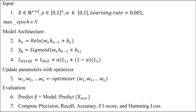
The HSSAE algorithm was trained using the hybrid loss function defined in Eq. 12, which combines BCE with \({L}_{1}\) and \({L}_{2}\) regularization to balance sparsity and stability. Model parameters, including weights and biases, were updated using the Adam optimizer with a learning rate of 0.001, \({\upbeta }_{1}=0.9\), \({\upbeta }_{2}=0.999\), and \(\epsilon ={10}^{-8}\). During training, data were processed in mini-batches according to the batch size of each dataset. For each batch, a forward pass computed the activations of the encoder, latent, and output layers, and the HSSAE loss was evaluated. Gradients were then calculated using backpropagation, and the parameters were updated iteratively with the Adam optimizer until convergence was achieved. After training, the model generated predictions on the test set, and performance was evaluated using Accuracy, Precision, Recall, F1-score, and Hamming Loss.
Empirical study on health indicator dataset
The HSSAE algorithm performance was evaluated using various classification metrics derived from the confusion matrix, as presented in Table 6. The model achieved an overall accuracy of 89%, demonstrating its effectiveness in distinguishing between diabetic and non-diabetic cases. For the negative class (non-diabetic), the model recorded a precision of 91%, a recall of 86%, and an F1-score of 88%. These metrics indicate the model’s ability to identify non-diabetic instances while maintaining a moderate false-negative rate correctly. In the positive class (diabetic), the HSSAE model achieved a precision of 86%, a recall of 92%, and an F1-score of 89%. This reflects the model’s proficiency in accurately detecting diabetic cases, striking a balance between precision and recall. The macro and weighted averages for precision, recall, and F1-score were all 89%, highlighting the model’s consistent performance across both classes. The HSSAE algorithm demonstrates a robust capability to differentiate between diabetic and non-diabetic cases, achieving high accuracy and balanced precision and recall across both classes.
Performance comparison with baseline models on the health indicator dataset
The HSSAE algorithm was comparatively evaluated against both machine learning and deep learning models on the Health Indicator dataset, with each model’s performance assessed across key metrics, including precision, recall, F1-score, accuracy, AUC, and Hamming loss. Table 7 compares the performance of the HSSAE model with traditional machine learning models, including Decision Trees (DT), Random Forest (RF), K-Nearest Neighbours (KNN), and Naive Bayes (NB). The HSSAE model outperforms all other classifiers, achieving an accuracy of 89%, a precision of 86%, and an AUC of 0.95. In comparison, models such as DT, RF, KNN, and NB show lower performance, with reduced F1-scores and accuracy, as well as higher Hamming losses. This highlights the HSSAE algorithm’s superior ability to predict health outcomes from sparse data.
Table 8 provides a comparison with deep learning models, such as CNN, LSTM, and SSAE. The HSSAE algorithm consistently outperformed these models in terms of precision, recall, F1-score, accuracy, and AUC. The HSSAE model achieved the highest F1-score (89%), precision (86%), and AUC (0.95), making it the most effective model for health data prediction, especially when compared to the lower performance of CNN, LSTM and SAE.
Comparison with SSAE + Machine learning model on health indicator dataset
Table 9 shows the hybrid approach of SSAE combined with traditional machine learning models. Again, the HSSAE algorithm outperforms the others, achieving a high accuracy of 89%, a precision of 86%, and an AUC of 0.95, considerably higher than the combinations of SSAE and machine learning classifiers.
Figure 11 presents the ROC-AUC and Precision-Recall curves for the proposed HSSAE algorithm. The model achieved an AUC score of 0.95 and a Precision-Recall curve score of 0.91, demonstrating its strong ability to distinguish between positive and negative cases. These curves illustrate the model’s outstanding performance in diabetes detection, highlighting high sensitivity and specificity.

ROC-AUC & precision-recall curve for health indicator dataset.
Empirical study on EHRs diabetes prediction dataset
The HSSAE algorithm model exhibited strong performance on the EHRs Diabetes Prediction Dataset, as detailed in Table 10. The model achieved an accuracy of 93%, indicating its effectiveness in distinguishing between diabetic and non-diabetic cases. For the negative class (non-diabetes), the model attained a precision of 95%, a recall of 92%, and an F1-score of 93%. These metrics demonstrate the model’s proficiency in correctly identifying non-diabetic instances while minimizing false negatives. In the positive class (diabetes), the model achieved a precision of 92%, a recall of 95%, and an F1-score of 94%. This reflects the model’s capability to accurately detect diabetic cases with a balanced approach between precision and recall. The macro and weighted averages for precision, recall, and F1-score were all 93%, further emphasizing the model’s consistent performance across both classes. The HSSAE model demonstrates a robust ability to differentiate between diabetic and non-diabetic cases, achieving high accuracy and balanced precision and recall across both classes.
Comparison with baseline models on EHRs diabetes prediction dataset
Table 11 compares the performance of the HSSAE algorithm with traditional machine learning classifiers, including DT, RF, KNN, and NB, on the EHRs Diabetes Prediction Dataset. The HSSAE model consistently outperformed all other classifiers, achieving the highest precision (92%), recall (95%), and F1-score (94%). Additionally, the HSSAE model achieved an impressive AUC of 0.99, indicating its strong ability to differentiate between positive and negative classes. In contrast, the traditional machine learning models, such as DT, RF, and KNN, showed lower performance with reduced F1-scores and accuracy, along with higher Hamming losses. This highlights the HSSAE model’s superior accuracy and effectiveness in diabetes prediction.
Table 12 further compares the HSSAE algorithm with top-performing deep learning models, including CNN, LSTM, and SSAE. The HSSAE model outshines these models across all performance metrics, achieving the highest F1-score (94%), precision (92%), and AUC (0.99). The HSSAE model also demonstrated superior recall and accuracy, establishing it as a more robust and efficient model for predicting diabetes, particularly in healthcare datasets with sparse data. In comparison, models such as CNN and LSTM reported lower precision, recall, and F1-scores, demonstrating the HSSAE model’s effectiveness in handling complex healthcare data.
Comparison with SSAE + ML models on EHRs diabetes prediction dataset
The HSSAE algorithm is compared with hybrid SSAE + machine learning models, including SSAE + DT, SSAE + RF, SSAE + KNN, and SSAE + NB, as presented in Table 13. The HSSAE algorithm outperformed all evaluation metrics, including precision, recall, F1-score, and accuracy. Furthermore, the Hamming loss for HSSAE is significantly lower (0.07), indicating fewer misclassifications and enhancing the model’s reliability in real-world applications. The hybrid SSAE + machine learning models performed well but were outperformed by the HSSAE model, confirming its superiority.
In Fig. 12, the ROC-AUC and Precision-Recall curves for the HSSAE algorithm are shown. The model achieved an AUC score of 0.99 and a Precision-Recall curve score of 0.95, indicating an exceptional ability to differentiate between positive and negative cases. These curves highlight the model’s outstanding performance in diabetes detection, with excellent sensitivity and specificity.

ROC-AUC & Precision-Recall Curve for EHRs Diabetes prediction dataset.
Impact of alpha (\(\boldsymbol{\alpha }\)) in the loss function
The impact of the α parameter in the loss function was evaluated by testing three values: \(\alpha\)= 0 (Pure \({\text{L}}_{2}\) regularization), optimized \(\alpha\)(best performing), and \(\alpha\)= 1 (Pure \({\text{L}}_{1}\) regularization) for each dataset. The results are presented in Tables 14, 15.
The results, as summarized in Tables 14, 15, highlight the critical role of \(\alpha\) in determining the model’s classification performance across different datasets. Relying solely on \({\text{L}}_{1}\) regularization (\(\alpha\) = 1) introduces excessive sparsity, leading to a decline in overall model generalization. Conversely, pure \({\text{L}}_{2}\) regularization (\(\alpha\) = 0) promotes stability but lacks the feature selection capability for optimal classification. The best performance is consistently observed at optimized \(\alpha\) values, confirming that an appropriate balance between \({\text{L}}_{1}\) and \({\text{L}}_{2}\) regularization enhances feature selection, model robustness, and overall classification accuracy.
Uncertainty quantification and error analysis
The reliability and robustness of the HSSAE algorithm were evaluated through uncertainty quantification and detailed misclassification analysis using confusion matrices for both datasets. These analyses provide a comprehensive understanding of model performance, variability, and potential weaknesses.
Confidence intervals
The 95% confidence interval for classification accuracy was calculated using the standard formula for proportions as presented in Eq. (22).
where, \(\widehat{p}\) is the observed accuracy, \(n\) is the number of test samples, and 1.96 corresponds to the 95% confidence level.
Health Indicator Dataset:
-
Total instances: 131,001
-
Accuracy = 0.8873 (95% CI: [0.8856, 0.8890])
EHRs Diabetes Prediction Dataset:
-
Total instances: 54,900
-
Accuracy = 0.9338 (95% CI: [0.9318, 0.9359])
The narrow confidence intervals indicate low variability, demonstrating that the model’s performance is stable and unlikely to be attributable to random chance, which is critical for healthcare applications.
Misclassification analysis
To better understand the model’s misclassifications, we present the confusion matrix for each dataset, highlighting the distribution of true positives, true negatives, false positives, and false negatives. This provides insights into the model’s performance and areas where errors are more likely to occur.
Health Indicator Dataset:
-
Misclassified 14.4% of negative cases (class 0) as positive.
-
Misclassified 8.1% of positive cases (class 1) as negative.
EHRs Diabetes Prediction Dataset:
-
Misclassified 8.3% of negative cases (class 0) as positive.
-
Misclassified 4.9% of positive cases (class 1) as negative.
This analysis highlights weaknesses specific to certain classes, showing that errors are somewhat higher in negative cases. Recognizing these patterns can guide targeted feature engineering or class-specific regularization in future model improvements.
Visualization of misclassifications
To further illustrate misclassification patterns, confusion matrix heatmaps were generated for both datasets (Fig. 13). The heatmaps confirm that misclassifications are more frequent in negative cases (class 0), complementing the numerical analysis.

Confusion matrix heatmaps of true and predicted labels.
The uncertainty quantification and misclassification analysis performed in this study are especially important in healthcare settings, where predictive errors can have significant clinical consequences. By providing confidence intervals and outlining class-specific misclassification patterns, the HSSAE algorithm shows both strong overall performance and transparency in its predictions. These analyses enable healthcare practitioners to make a more informed assessment of model reliability, thereby enhancing trust, interpretability, and safety in clinical decision-making.
Discussion
The HSSAE algorithm demonstrated significant effectiveness in distinguishing between diabetic and non-diabetic cases. On the Health Indicator Dataset, the proposed algorithm achieved an overall accuracy of 89%, with a precision of 91%, a recall of 86%, and an F1-score of 88% for the non-diabetic class. For the diabetic class, it attained a precision of 86%, a recall of 92%, and an F1-score of 89%, as detailed in Table 6. These consistent macro and weighted averages of 89% underscore the algorithm’s reliability in classification tasks.
The superiority of the HSSAE algorithm becomes evident when compared to traditional machine learning models in terms of performance and reliability. As presented in Table 7 HSSAE achieved an AUC of 0.95, surpassing Decision Trees (DT) with an AUC of 0.78, Random Forest (RF) with 0.84, K-Nearest Neighbours (KNN) with 0.84, and Naive Bayes (NB) with 0.71. Additionally, HSSAE reported a lower Hamming loss of 0.11, indicating fewer misclassification errors than competing models. This suggests that the proposed algorithm, HSSAE, enhances predictive accuracy and reduces the likelihood of mistakes. In comparison with other deep learning architectures, such as CNN, Long Short-Term Memory networks (LSTM), and Stacked Sparse Autoencoders (SSAE), HSSAE consistently outperformed its counterparts. Table 8 shows that, HSSAE achieved higher precision (86%), recall (92%), and F1-score (89%) compared to CNN’s precision of 73%, recall of 78%, and F1-score of 75%, as well as LSTM’s precision of 72%, recall of 84%, and F1-score of 78%. Further, HSSAE’s AUC of 0.95 exceeded CNN’s 0.73 and LSTM’s 0.84, underscoring its robust capability in diabetes prediction. Furthermore, the analysis involved hybrid models combining SSAE with traditional machine learning classifiers, which demonstrated commendable performance; however, they failed to surpass the HSSAE algorithm. For instance, SSAE combined with RF achieved an AUC of 0.91, still lower than HSSAE’s 0.95, reinforcing the latter’s efficacy, as presented in Table 9.
Extending the evaluation to the EHRs Diabetes Prediction Dataset, the HSSAE algorithm continued to demonstrate exceptional performance. The algorithm achieved an accuracy of 93%, with the non-diabetic class recording a precision of 95%, a recall of 92%, and an F1-score of 93%. In the diabetic class, the algorithm achieved an accuracy of 92%, a recall of 95%, and an F1-score of 94%. Both the macro and weighted averages reached 93%, reflecting the proposed algorithm’s balanced and dependable performance across both classes, as shown in Table 10. A comparative analysis of the proposed algorithm, HSSAE, against traditional machine learning models on the second dataset highlights the superior performance of HSSAE. Achieving the highest precision (92%), recall (95%), F1-score (94%), and AUC (0.99), the HSSAE algorithm reported a notably low Hamming loss of 0.07, reflecting its accuracy and reliability in diabetes prediction, as shown in Table 11. When evaluated against other deep learning models on the EHRs dataset, HSSAE maintained its superior performance. Notably, HSSAE’s F1-score of 94% was significantly higher than those of CNN (65%) and LSTM (72%), emphasizing its effectiveness in balancing precision and recall, as indicated in Table 12. Hybrid models combining SSAE with traditional machine learning classifiers were also assessed on the EHRs dataset. While these models performed well, the HSSAE algorithm consistently outperformed them, reinforcing its robustness and applicability in real-world scenarios, as presented in Table 13.
The impact of the regularization parameter α in the loss function was examined by evaluating three different values:\(\alpha =0\) (pure \({\text{L}}_{2}\) regularization), optimized \(\alpha\) (best performing), and \(\alpha =1\) (pure \({\text{L}}_{1}\) regularization). The results, summarized as shown in Tables 14, 15, highlight the critical role of α in determining the proposed algorithm’s classification performance across two different datasets. Using only \({\text{L}}_{1}\) regularization (α = 1) resulted in excessive sparsity, which negatively affected the model’s generalization performance. Conversely, pure \({\text{L}}_{2}\) Regularization (\(\alpha =0\)) promoted stability but lacked the feature selection capability needed for optimal classification. The best performance was consistently observed at optimized α values, confirming that an appropriate balance between \({\text{L}}_{1}\) and \({\text{L}}_{2}\) regularization enhances feature selection, model robustness, and overall classification accuracy.
The empirical evaluations confirm that the HSSAE algorithm excels in distinguishing diabetic from non-diabetic cases, consistently outperforming traditional ML and DL baselines across multiple metrics. Its capacity to manage sparse and high-dimensional data, reinforced by robust regularization strategies, highlights its potential as a reliable tool for accurate and timely diabetes prediction in clinical practice. Although developed as a static model, the HSSAE algorithm can be adapted for longitudinal applications to achieve functionality comparable to that of temporal architectures, such as LSTM. Furthermore, for multi-modal learning, modality-specific encoders (structured EHRs, medical imaging, clinical text) can be integrated to extract domain-relevant representations that are subsequently fused in a shared latent space. For temporal datasets, recurrent models such as LSTM or GRU, as well as temporal self-attention mechanisms, can be embedded within the HSSAE algorithm to capture sequential dependencies in longitudinal patient records. In a clinical context, the HSSAE algorithm could be deployed in several real-world scenarios. In primary care, it may support physicians by flagging high-risk patients using routinely collected EHR data, enabling early intervention. In hospital settings, integration into electronic health record systems could allow continuous monitoring of patient trajectories and prediction of adverse outcomes. In telemedicine and remote monitoring platforms, HSSAE algorithm could analyze longitudinal data to inform personalized care plans for diabetic patients. These scenarios highlight the practical applicability of the HSSAE algorithm in providing enhanced decision support across various healthcare settings. Several challenges must be addressed before clinical deployment can occur. Ethical concerns regarding bias and fairness remain critical, as predictive performance may vary across demographic subgroups. Interpretability is a further limitation, since deep learning models are often perceived as “black boxes,” highlighting the need for explainable AI techniques to foster clinician trust. Additionally, the handling of sensitive health records necessitates strict adherence to privacy and security standards. Finally, external validation across diverse populations is essential to ensure generalizability, as performance may differ when applied beyond the datasets used in this study.
Conclusion
In the healthcare field, where every prediction can have significant implications for patient outcomes, the accuracy and reliability of predictive models are of utmost importance. The proposed HSSAE algorithm demonstrated superior performance in predicting Type 2 diabetes, outperforming traditional machine learning and deep learning models in key metrics, including precision, recall, F1-score, accuracy, and AUC. The results indicate that HSSAE is highly effective for identifying diabetes, especially in sparse and high-dimensional datasets, while maintaining low misclassification rates. This highlights its potential as a practical and dependable tool for clinical decision support, particularly in scenarios involving sparse and high-dimensional medical data. Despite its promising results, the HSSAE algorithm’s performance is susceptible to the choice of the α parameter in the hybrid loss function. This necessitates careful tuning to find the optimal balance between \({L}_{1}\) and \({L}_{2}\) regularization. Additionally, the model’s effectiveness can vary depending on the sparsity and dimensionality of the dataset, underscoring the need for further optimization. The performance may also be influenced by the dataset type, requiring more rigorous evaluation on diverse, large-scale datasets. Furthermore, while the model performs well on the datasets tested, its generalization to other healthcare problems and data types remains an area for improvement.
Future research will prioritize the external validation of HSSAE using large-scale, non-Kaggle datasets such as MIMIC-III or NHANES to evaluate generalizability and clinical relevance across diverse populations. Model explainability will also be addressed through integration of SHAP, LIME, or attention-based interpretability methods to clarify feature importance and enhance transparency for clinical adoption. In addition, a more rigorous evaluation framework will be implemented, including the computation of p-values and k-fold cross-validation, to establish the statistical significance and robustness of performance gains. These directions will strengthen the reliability, interpretability, and applicability of HSSAE in real-world healthcare scenarios.
Data availability
The data used in this study are available from the corresponding author upon reasonable request.
Code availability
The code developed for data analysis and to support the findings of this study is available upon request from the corresponding author.
References
Alazwari, A. et al. Predicting the development of T1D and identifying its Key Performance Indicators in children; a case-control study in Saudi Arabia”. PLoS ONE 18(3), 1–26. https://doi.org/10.1371/journal.pone.0282426 (2023).
Khunti, K., et al. Current global health challenge diabetes and multiple long-term conditions: A review of our current global health challenge. 46(12), 2092–2101 (2023).
Tecce, N., Pivonello, R., Menafra, D., Progan, M. & Colao, A. Human nutrition & metabolism diet and gut microbiome: Impact of each factor and mutual interactions on prevention and treatment of type 1, type 2, and gestational diabetes mellitus. Human Nutr. Metab. 38(August), 200286. https://doi.org/10.1016/j.hnm.2024.200286 (2024).
Chaki, J., Thillai Ganesh, S., Cidham, S. K. & Ananda Theertan, S. Machine learning and artificial intelligence based Diabetes Mellitus detection and self-management: A systematic review. J. King Saud Univ. Comput. Inf. Sci. 34(6), 3204–3225. https://doi.org/10.1016/j.jksuci.2020.06.013 (2022).
Luekhong, P. Advancing book recommendation systems: A comparative analysis of collaborative filtering and matrix factorization algorithms. J. Inf. Syst. Eng. Manag. 10(4s), 215–225. https://doi.org/10.52783/jisem.v10i4s.492 (2025).
Zhang, Y., Chen, H., Xiang, S. & Lv, Z. Identification of DNA N6-methyladenine modifications in the rice genome with a fine-tuned large language model. Front. Plant Sci. https://doi.org/10.3389/fpls.2025.1626539 (2025).
Alkaabi, H., Jasim, A. K. & Darroudi, A. From static to contextual: A survey of embedding advances in NLP. PERFECT J. Smart Algorithms. 2(2), 57–66. https://doi.org/10.62671/perfect.v2i2.77 (2025).
Karim, I., Daud, H. B., Zainuddin, N. & Sokkalingam, R. Addressing limitations of the K-means clustering algorithm: Outliers, non-spherical data, and optimal cluster selection. AIMS Math. 9(July), 25070–25097. https://doi.org/10.3934/math.20241222 (2024).
Ekundayo, F. Machine learning for chronic kidney disease progression modelling: Leveraging data science to optimize patient management. World J. Adv. Res. Rev. 24(03), 453–475. https://doi.org/10.30574/wjarr.2024.24.3.3730 (2024).
Chang, V., Ganatra, M. A., Hall, K., Golightly, L. & Xu, Q. A. An assessment of machine learning models and algorithms for early prediction and diagnosis of diabetes using health indicators. Healthcare Anal. 2(October), 100118. https://doi.org/10.1016/j.health.2022.100118 (2022).
Zubair, M., Rais, H. & Alazemi, T. A novel attention-guided enhanced U-Net with hybrid edge-preserving structural loss for low-dose CT image denoising. IEEE Access. 13(January), 6909–6923. https://doi.org/10.1109/ACCESS.2025.3526619 (2025).
Rayed, E. et al. Informatics in medicine unlocked deep learning for medical image segmentation: State-of-the-art advancements and challenges. Inform. Med. Unlocked. 47(January), 101504. https://doi.org/10.1016/j.imu.2024.101504 (2024).
Zubair, M., Rais, H. B., Ullah, F., Faheem, M. & Khan, A. A. Enabling predication of the deep learning algorithms for low-dose CT scan image denoising models: A systematic literature review. IEEE Access. 12(May), 79025–79050. https://doi.org/10.1109/ACCESS.2024.3407774 (2024).
Katsarou, D. N., Georga, E. I., Christou, M. A., Christou, P. A. & Tigas, S. Optimizing hypoglycaemia prediction in type 1 diabetes with Ensemble Machine Learning modeling. BMC Med. Inform. Decis Mak. https://doi.org/10.1186/s12911-025-02867-2 (2025).
Chowdary, M. K. An expert system for insulin dosage prediction using machine learning & deep learning algorithms. in 2023 8th International Conference on Communication and Electronics Systems (ICCES) no. Icces 1291–1297 (2023). https://doi.org/10.1109/ICCES57224.2023.10192778.
Keshtkar, A., Ayareh, N. & Atighi, F. Artificial intelligence in diabetes management: Revolutionizing the diagnosis of diabetes mellitus, A literature review. Shiraz E-Medical J. 25, e146903. https://doi.org/10.5812/semj-146903 (2024).
Pathak, P. & Elchouemi, A. Predicting early phase of type 2 diabetic by deep learning. in CITISIA 2020—IEEE Conference on Innovative Technologies in Intelligent Systems and Industrial Applications, Proceedings (2020). https://doi.org/10.1109/CITISIA50690.2020.9371843.
Zhang, Q., Zhou, J. & Zhang, B. A noninvasive method to detect diabetes mellitus and lung cancer using the stacked sparse autoencoder PAMI Research Group , Department of Computer and Information Science , University of Macau. in ICASSP 2020 - 2020 IEEE International Conference on Acoustics, Speech and Signal Processing (ICASSP) 1409–1413 (2020).
Kannadasan, K., Edla, D. R. & Kuppili, V. Type 2 diabetes data classification using stacked autoencoders in deep neural networks. Clin. Epidemiol. Glob Health. 7(4), 530–535. https://doi.org/10.1016/j.cegh.2018.12.004 (2019).
Alex, S. A., Nayahi, J. J. V., Shine, H. & Gopirekha, V. Deep convolutional neural network for diabetes mellitus prefile:///C:/Users/ABDUSSAMAD/OneDrive—Universiti Teknologi PETRONAS/Desktop/new Lit/213.pdfdiction. Neural Comput. Appl. 34(2), 1319–1327. https://doi.org/10.1007/s00521-021-06431-7 (2022).
Vivekanandan, A. & Shanmugam, A. K. Stacked Autoencoder for Diabetes Classification (Springer, 2020). https://doi.org/10.1007/978-981-16-2406-3.
García-Ordás, M. T., Benavides, C., Benítez-Andrades, J. A., Alaiz-Moretón, H. & García-Rodríguez, I. Diabetes detection using deep learning techniques with oversampling and feature augmentation. Comput. Methods Programs Biomed. https://doi.org/10.1016/j.cmpb.2021.105968 (2021).
Thaiyalnayaki, K. Classification of diabetes using deep learning and svm techniques. Int. J. Curr. Res. Rev. 13(1), 146–149. https://doi.org/10.31782/IJCRR.2021.13127 (2021).
Miotto, R., Li, L., Kidd, B. A. & Dudley, J. T. Deep Patient: An unsupervised representation to predict the future of patients from the electronic health records. Sci. Rep. 6(April), 1–10. https://doi.org/10.1038/srep26094 (2016).
Chetoui, M. & Akhloufi, M. A. Federated learning for diabetic retinopathy detection using vision transformers, 948–961 (2023).
Lan, E. Long-Range Vascular Signals, vol. c.
Dhyaneshwar, K. M., Sri, A. S., Srikanth, B. K., Naveen, N. S. & Rhevathi, M. Knowledge graph-based effective cardiovascular disease treatment using BEHRT: A deep learning approach with EHR integration. in 2025 International Conference on Data Science, Agents and Artificial Intelligence, ICDSAAI 2025, Institute of Electrical and Electronics Engineers Inc. (2025). https://doi.org/10.1109/ICDSAAI65575.2025.11011824.
Wang, H. et al. Enhancing predictive accuracy for urinary tract infections post-pediatric pyeloplasty with explainable AI: An ensemble TabNet approach. Sci. Rep. 15, 1. https://doi.org/10.1038/s41598-024-82282-1 (2025).
Li, W. TabNet for high-dimensional tabular data: advancing interpretability and performance with feature fusion. in IET Conference Proceedings CP915, IET 168–173 (2025).
Emami, M., Parthe, M. S., Sundeep, P. & Alyson, R. Generalization error of generalized linear models in high dimensions (2019).
Profile, S. E. E. Deep learning applied to regression, classification and feature transformation problems e Ram, (2022).
Halder, R. K., Uddin, M. N., Uddin, A. & Aryal, S. Enhancing K—nearest neighbor algorithm: A comprehensive review and performance analysis of modifications. J. Big Data https://doi.org/10.1186/s40537-024-00973-y (2024).
Ambhika, C. & Sheena, B. G. Enhancing predictive modeling in high dimensional data using hybrid feature selection. in 2024 5th International Conference on Electronics and Sustainable Communication Systems (ICESC), no. Icesc 873–879 (2024). https://doi.org/10.1109/ICESC60852.2024.10690153.
Moghadam, M. P., Moghadam, Z. A., Reza, M., Qazani, C., Plawiak, P. & Alizadehsani, R. Impact of Artificial Intelligence in Nursing for Geriatric Clinical Care for Chronic Diseases: A Systematic Literature Review, vol. 12, no. September (IEEE, 2024). https://doi.org/10.1109/ACCESS.2024.3450970.
Jabason, E., Member, S., Ahmad, M. O. & Swamy, M. N. S. Missing structural and clinical features imputation for semi-supervised Alzheimer’s disease classification using stacked sparse autoencoder. in 2018 IEEE Biomedical Circuits and Systems Conference (BioCAS) 1–4 (2018).
Nazir, N., Sarwar, A. & Singh, B. Recent developments in denoising medical images using deep learning: An overview of models, techniques, and challenges. Micron 180, 103615. https://doi.org/10.1016/j.micron.2024.103615 (2024).
Shen, X. et al. A brief review on deep learning applications in genomic studies. Front. Syst. Biol. 2, 877717. https://doi.org/10.3389/fsysb.2022.877717 (2022).
Houssein, E. H., Mohamed, R. E. & Ali, A. A. Machine learning techniques for biomedical natural language processing: A comprehensive review. IEEE Access 9, 140628–140653. https://doi.org/10.1109/ACCESS.2021.3119621 (2021).
Jiang, X., Hu, Z., Wang, S. & Zhang, Y. Deep learning for medical image-based cancer diagnosis (2023).
Kauffman, J. et al. Embedding methods for electronic health record research modelling. 39, 24. https://doi.org/10.1146/annurev-biodatasci-103123 (2025).
Hama, T. et al. Enhancing patient outcome prediction through deep learning with sequential diagnosis codes from structured electronic health record data: Systematic review. J. Med. Internet Res. 27, e57358. https://doi.org/10.2196/57358 (2025).
Jiang, J.-P., Liu, S.-Y., Cai, H.-R., Zhou, Q. & Ye, H.-J. Representation learning for tabular data: A comprehensive survey (2025). Available: http://arxiv.org/abs/2504.16109
Li, H. et al. A machine learning-based prediction of hospital mortality in mechanically ventilated ICU patients. PLoS ONE 19(9), e0309383. https://doi.org/10.1371/journal.pone.0309383 (2024).
Harvey, H. B. & Sotardi, S. T. The pareto principle. J. Am. Coll. Radiol. 15(6), 931. https://doi.org/10.1016/j.jacr.2018.02.026 (2018).
Sun, P., Wang, Z., Jia, L. & Xu, Z. SMOTE-kTLNN: A hybrid re-sampling method based on SMOTE and a two-layer nearest neighbor classifier. Expert Syst. Appl. 238, 121848. https://doi.org/10.1016/j.eswa.2023.121848 (2024).
Mahmood, Z., Safran, M., Alfarhood, S. & Ashraf, I. Algorithmic and mathematical modeling for synthetically controlled overlapping, 1–22 (2025).
Berahmand, K., Daneshfar, F., Sadat, E. & Yuefeng, S. Autoencoders and their Applications in Machine Learning: A Survey (Springer, 2024). https://doi.org/10.1007/s10462-023-10662-6.
Abdussamad, A. et al. Regularized stacked autoencoder with dropout-layer to overcome overfitting in numerical high-dimensional sparse data. J. Adv. Res. Des. 129(1), 60–74 (2025).
Alberti, M., Seuret, M., Ingold, R. & Liwicki, M. A pitfall of unsupervised pre-training extended abstract.
Han, G. Effective feature extraction via stacked sparse autoencoder to improve intrusion detection system. IEEE Access 6, 41238–41248. https://doi.org/10.1109/ACCESS.2018.2858277 (2018).
Le, T. T. H., Kim, J. & Kim, H. An effective intrusion detection classifier using long short-term memory with gradient descent optimization. in 2017 International Conference on Platform Technology and Service, PlatCon 2017 - Proceedings, no. February (2017). https://doi.org/10.1109/PlatCon.2017.7883684.
Zhang, Z. Improved adam optimizer for deep neural networks. in 2018 IEEE/ACM 26th International Symposium on Quality of Service, IWQoS 2018 1–2 (2019). https://doi.org/10.1109/IWQoS.2018.8624183
Acknowledgements
The authors gratefully acknowledge the financial support provided by the YUTP-FRG Grant under the cost centre: 015LC0-442, Universiti Teknologi PETRONAS, Malaysia. They also deeply appreciate the anonymous editors and peer reviewers for their meticulous revisions and invaluable feedback.
Author information
Authors and Affiliations
Contributions
(1) Abdussamad developed the research methodology and designed the Hybrid Stacked Sparse Autoencoder (HSSAE) model. He conducted data preprocessing, implemented machine learning and deep learning models, performed the experiments, and prepared the initial draft of the manuscript. (2) Hanita Daud and (3) Rajalingam Sokkalingam supervised the research, provided methodological guidance, and critically reviewed the manuscript. (4) Muhammad Zubair, (5) Iliyas Karim Khan, and (6) Zafar Mahmood contributed to reviewing the manuscript and refining the final version.
Corresponding author
Ethics declarations
Competing interests
The authors declare no competing interests.
Additional information
Publisher’s note
Springer Nature remains neutral with regard to jurisdictional claims in published maps and institutional affiliations.
Rights and permissions
Open Access This article is licensed under a Creative Commons Attribution-NonCommercial-NoDerivatives 4.0 International License, which permits any non-commercial use, sharing, distribution and reproduction in any medium or format, as long as you give appropriate credit to the original author(s) and the source, provide a link to the Creative Commons licence, and indicate if you modified the licensed material. You do not have permission under this licence to share adapted material derived from this article or parts of it. The images or other third party material in this article are included in the article’s Creative Commons licence, unless indicated otherwise in a credit line to the material. If material is not included in the article’s Creative Commons licence and your intended use is not permitted by statutory regulation or exceeds the permitted use, you will need to obtain permission directly from the copyright holder. To view a copy of this licence, visit http://creativecommons.org/licenses/by-nc-nd/4.0/.
About this article

Cite this article
Abdussamad, Daud, H., Sokkalingam, R. et al. A deep learning framework with hybrid stacked sparse autoencoder for type 2 diabetes prediction. Sci Rep 15, 36678 (2025). https://doi.org/10.1038/s41598-025-20534-4
Received:
Accepted:
Published:
Version of record:
DOI: https://doi.org/10.1038/s41598-025-20534-4
