
Abstract
The spin-statistics theorem leads to Pauli’s Exclusion Principle (PEP), the basis of the stability of matter and many other phenomena relevant to physics, astrophysics, cosmology, and even biology. Possible violations of the PEP (PEPV) have been searched for since its inception; they may come from various Beyond Standard Model descriptions, including Non-Commutative Quantum Gravity models and extensions of the Quantum Field Theory, which must follow the Messiah-Greenberg Super-Selection (MGSS) rule and lead to the Quon description of the spin-statistic symmetries: the parastatstics. Efforts to search for a PEPV are not new; however, they have typically measured those cases without respecting MGSS. VIP (VIolation of the Pauli exclusion principle) first and its successor VIP-2, both sited in the “Gran Sasso underground laboratory,” aimed to set the most stringent limit for the non-Paulian transition following the MGSS rule. After two years of data with VIP-2 and better modeling of the electron-atom interaction, we present the most stringent upper limit of the probability of PEP violation for this case (\(\beta ^{2}/2<2.47\times 10^{-43}\)), thus completing the state-of-the-art of all possible PEPV cases, and the consequent constraint to the Quon description: \(1+q < 4.94 \times 10^{-43}\).
Introduction
As a fundamental pillar of quantum mechanics for explaining the atomic structure and, consequently, the stability of matter1, Wolfgang Pauli formulated the Pauli Exclusion Principle (PEP) in 1925. It forms the basis of the periodic table of elements, electric conductivity in metals, and the degeneracy pressure, which makes white dwarf and neutron stars stable. The PEP is a direct implication of the Spin-Statistics Theorem (SST)2, grouping the particles in the Standard Model into two categories: the bosons with integer spin and the fermions with half-integer spin. Within Quantum Field Theory (QFT), they transform differently by exchanging identical particles: bosonic states have symmetrical permutations, and fermionic ones have antisymmetrical3. Even though the PEP is connected to many fundamental phenomena, an intuitive explanation is still missing4.
The PEP prohibits two electrons from simultaneously occupying the same atomic energy level in a given system. A violation of the PEP (PEPV) could potentially occur in the framework of theories beyond the Standard Model (e.g.,5). Intriguing and testable examples come from the Non-Commutative Quantum Gravity (NCQG) models as per \(\theta\)-Poincaré6,7,8.
Another class of theories is related to the nature of the particles, for example, the paronic field proposed by Greenberg and Mohapatra9,10,11, for which particles have ranks. When two anti-symmetric particles with the same rank form a symmetric system, they adhere to the Pauli exclusion principle; the fermionic field belongs to the lowest rank, while the so-called parafermionic to higher ranks. The same distinction is valid for bosonic and parabosonic fields. Within this description, a paronic field is a mixture of particles (fermions or bosons) and paraparticles (parafermions or parabosons). A recent work12 presented a variant in which a third class of particles (distinct from fermions and bosons) can exist as a parastatistic.
For this class of theories, Messiah and Greenberg have proved an absolute selection rule13, the “Messiah-Greenberg Super-Selection” (MGSS), which forbids transitions among states with different symmetries (i.e., ranks) for a given system. In other words, a parafermion cannot become a fermion and vice versa. That makes parafermions distinguishable experimentally from regular-behaving particles by, for example, testing the PEPV on fermions: any violation implies the presence of an electron with parafemionic symmetry. This work tests the PEP of electrons in atomic transitions.
Classification of the Pauli exclusion principle violation cases
The work in14 identifies three types of processes for distinguishing a PEPV occurrence with electron atomic transitions, schematized in Fig. 1:

Scheme of the Type I, II, and III transition processes and signature emission (see Sect. 1.1). In the atom depiction, nuclei are in red, electrons of the system in cyan, newly introduced electrons in green, positrons in purple, and emitted X-rays in yellow. For simplicity, we depicted the atomic levels of interest for this work involved in the K\(\phantom{0}_\alpha\) transition with the s-orbital of the ground state represented by an inner circle with two electrons (fully occupied) and the non-ground states simplified as an external circle with an electron octet.
-
I
An electron that has not yet interacted with any other electron: e.g., a newly created electron from a pair-production as shown in the leftmost drawing of Fig. 1, experimentally pioneered by Goldhaber15;
-
II
An electron that has not yet interacted with a specific system: e.g., an electron injected in a solid—i.e., that is not part of its established atomic structure—that can test atom by atom (central drawing in Fig. 1), experimentally pioneered by Ramberg and Snow16;
-
III
An electron in a given system makes a forbidden transition, as shown in the rightmost drawing of Fig. 1, e.g., due to a new interaction force (for example, quantum gravity). Reines and Sobel pioneered this experimentally17.
In contrast to Type I and II experiments, which were conceived to test PEPV by respecting the MGSS rule, Type III tests violate this superselection and cannot be used, e.g., to test parastatistics. The measurement presented in this work belongs to Type II and delivers the strongest bound ever on the PEPV probability, which fulfills the MGSS, and a test for the parastatistical model “Quon”.
The Quon description for the Type II case
Several attempts to build consistent local quantum field theories9,18,19,20 culminated in the “Quon model”11,21,22,23, as a description with Fermi and Bose statistics interpolated. The Quon algebra is determined by the relation:
with \(a^{\dagger }\) and a, the ladder operators; q ranges between -1 and 1 and allows all representations of the symmetric group: \(q = -1\) corresponds to the fully antisymmetric representation (Fermi-Dirac statistics), while for \(q = 1\), the fully symmetric (Bose-Einstein statistics).
If a small violation of Fermi statistics is allowed, a state \(\beta \left| \text {PEPV}\right\rangle\) (\(\beta\) its coefficient) is introduced. Therefore, its probability of occurring in a system with two electrons in a symmetric state is \(\beta ^{2}/2\). With the Quon algebra, the interpretation is
In other words, \(\beta ^{2}\) is the coefficient of an anomalous component of the two-identical-fermions density matrix:
with \(\rho _a\) and \(\rho _s\) its antisymmetric and symmetric form, respectively.
Searching for Type II signature
The aforementioned pioneering experiment to search for a PEPV of Type II was performed in 1988 by Ramberg and Snow16, employing a dynamic test with electrons. The experiment searched for X-rays originating from Pauli-forbidden atomic transitions from the 2p to the fully occupied 1s ground state, i.e., the PEPV K\({}_\alpha\) transition, which would point to a violation of the PEP (schematized in Fig. 2). The crucial advantage of this type of experiment is the introduction of electrons, new to the system, by a direct electric current into a conductor: an “Open System” experiment. As per Type II, these “new” electrons are fermions testing different fermionic systems (atoms) with no previous interaction, checking all possible occupancy.

Schematic of PEP-allowed and PEP-violating K\({}_\alpha\) transition, respectively, on the left and the right. Reproduced from24.
The number of measured X-rays \(N_x\) emitted by the expected PEPV is estimated as follows25:
where \(\beta ^{2}/2\) is the PEPV probability, \(N_\textrm{new}\) is the total number of “new” conduction electrons injected into the system by the circulating current, and \(N_\textrm{int}\) is the minimum number of electron-atom encounters as electrons flow in the target, taking into account the conditions to reach the 2p state26. The “efficiency” considers the solid angle covered by the detector, the X-ray absorption in the target strip, and the detector sensitivity. The experiment of Ramberg and Snow set an upper limit for the probability that the PEP is violated for electrons of \(\beta ^{2}/2 < 1.7 \times 10^{-26}\). Following this pathfinder, the VIP experiment, the precursor of VIP-2, improved this limit by about two orders of magnitude27 and the experiment described in14 by one.
VIP-2 (VIolation of Pauli exclusion principle - 2) tests the Pauli Exclusion Principle (PEP) by injecting electrons in copper and measuring its atomic K\({}_\alpha\) transitions with high-precision X-ray detectors. Due to the extra shielding provided by the two electrons in the 1s state of the atom, the energy of the PEPV K\({}_\alpha\) atomic transition would be shifted down by about \(\sim 300\) eV. Therefore, with respect to the standard ones (from28, \(E^\textrm{Cu}_\mathrm {K\alpha 1} = 8047.78\) eV for K\({}_{\alpha 1}\) and \(E^\textrm{Cu}_\mathrm {K\alpha 2} = 8027.83\) eV for K\({}_{\alpha 2}\)), the energies of the PEPV are \(E_\textrm{PEPV} = 7746.73\) eV for K\({}_{\alpha 1}\) and 7728.92 eV for K\({}_{\alpha 2}\)29.
In the last two decades, many experiments have been carried out, setting upper limits for PEP violation probability30,31,32,33,34,35,36,37,38. These results were primarily obtained as by-products of experiments with different main scientific objectives (like Borexino36 and DAMA35). Some of these experiments investigate the PEP validity for composite particles like nucleons and nuclei, which is related to the stability of the atomic matter (i.e., equivalent to Type I and Type III). Experiments like VIP-2, however, investigate the atomic transitions of electrons, which are connected to the nature of elementary particles: they are the only Type II measurements.
The number of interactions
Given \(N_\textrm{new} = (1/e) I\Delta t\), where e is the electron charge, I the injected current intensity, and \(\Delta t\) is the duration of injection (i.e., how long the current is live), the probability of PEP violation is obtained from Eq. 4 as
Since \(N_x\) is the count of violating particles, all factors are clear and well-known except \(N_\textrm{int}\), which works as a normalization scale for \(\beta ^{2}/2\). It represents the average number of atoms encountered by the newly injected electrons.
In previous experiments, the average encounter probability was assumed due to the electron scattering along a linear path into the target, mostly because of phonons and lattice irregularities. However, several atoms are encountered from one scatter point to another. Therefore, that is a strong approximation and greatly underestimates the real encounters since it considers those atoms that scatter the electron. We recently introduced a new approach26.
Instead of relying on the average scatter distance, estimating the average time \(\tau _E\) between one encounter and another through diffusion-transport studies is more efficient. The modelization for a 1-D diffusion-transport model was done by applying a semi-classical approximation so as not to stray too far from the previous assumption: the estimated average encounter time is \(\tau _E \simeq 3.5\times 10^{-17}\) s. Calling \(T\propto nD/\,I\simeq 1.6\times 10^{3} /\, I\) the time an electron needs to be diffused across the entire target of dimension D with a density of electrons in the conducting band at a given temperature n26, \(N_\textrm{int} = T/\tau _E\simeq 4.6\times 10^{19} /\, I\); therefore, Eq. 5 is rewritten as follows:
VIP-2 apparatus
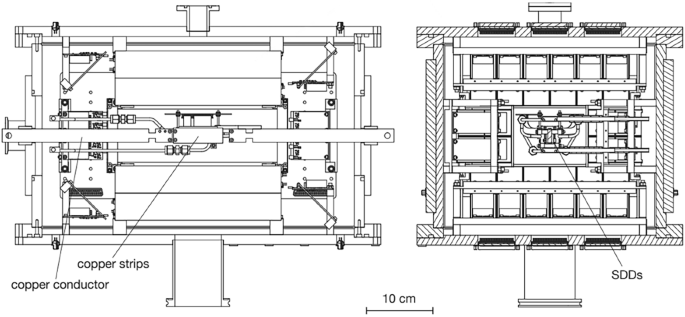
Schematic of the VIP-2 setup with, in evidence, the vacuum chamber, the targets (copper strips), the copper conductor used to inject current, and the SDDs; draw from39.
The VIP-2 experiment is schematized in Fig. 3. It comprises a vacuum chamber containing 32 Silicon Drift Detectors (SDDs) and two parallel copper strips as a target. The strips (76 mm \(\times\) 20 mm \(\times\) 25 \(\upmu\)m) are connected to a current generator (by the copper connectors in the figure): a current of 180 A circulates. Each parallel strip faces a matrix \(4\times 4\) of SDDs grouped electronically into two \(2\times 4\) arrays. Each SDD is 450 \(\upmu\)m thick with 0.64 cm\(\phantom{0}^{2}\) as active area (a total of 5.12 cm\(\phantom{0}^{2}\) for each array). The geometrical efficiency for the VIP-2 and the X-ray detection efficiency were calculated with a dedicated Monte Carlo Simulation built in GEANT4, taking into account all details of the geometrical distribution of the apparatus and target self-absorption. As a result, the “efficiency” reported in Eq. 4 is 7.25\(\times 10^{-2}\) for this experimental setup.
The vacuum chamber is evacuated at a pressure below \(10^{-5}\) mbar. It allows the SDDs to be cooled down safely to a temperature of 150 K by cryocooler. Six PT-100 sensors are installed inside to monitor SDDs and chamber temperatures. A cooling water circuit is installed on the copper strips to avoid a high rise in the target temperature when the current circulates, which would reduce the SDDs’ high-quality performance. The copper target is kept at a temperature of 20-25 \({}^{\circ }\)C. In these working conditions, SDDs provide an energy resolution for X-rays of about 190 eV Full-Width Half Maximum (FWHM) at 8 keV with a quantum efficiency of more than 99%. Such energy resolution can distinguish the PEP-forbidden copper K\(\phantom{0}_\alpha\) transition from the normal PEP-allowed in the energy spectra. SDD working principles and schemes are detailed in39.
To perform in situ SDD calibrations, a Fe-55 source is placed below the target covered by a 25 \(\upmu\)m thick Titanium foil. The K\(\phantom{0}_\alpha\) and K\(\phantom{0}_\beta\) lines emitted by Mn and Ti are used for each SDD calibration, translating their ADC counts into energy (in eV).
Since the experiment must be performed in a low background environment, it is sited underground at Gran Sasso underground laboratory (LNGS), in Italy, beneath about 1400 m of rock; it reduces the secondary Cosmic Rays flux by a factor of \(10^{6}\). A further external shielding is installed surrounding the VIP-2 vacuum chamber to reduce the natural background produced by the residual radioactivity of the rocks inside the LNGS cavern. This outer shielding consists of an inner layer of copper bricks and an exterior layer of lead blocks. A PT-100 sensor is installed on the external surface of the vacuum chamber to monitor the temperature within the passive shielding, kept fixed at 24 \({}^{\circ }\)C through an air cooling system.
Since April 2019, this final configuration of the VIP-2 experiment has been installed and took data continuously until May 2021.
Data

VIP-2 calibrated data in the region-of-interest 7000-8500 eV, of about two years of data taking (May 2019 to May 2021). The spectrum of the data acquired with a current circulating in the target is shown in blue. Data taken without current in the target, used as reference and control, shown in red. The copper and nickel K\({}_\alpha\) lines are visible in the spectra.
The analyzed data set corresponds to about two years of experimental operation, from May 2019 to May 2021. It amounts to 26916404 s (about 312 days) of data taking with current circulating and 27110263 s (about 314 days) without it. The first 2434602 s (about 28 days) of data taken with current were acquired with 150 A; subsequently, the nominal 180 A was used.
Calibration is performed in data blocks of a fixed length of ten days to minimize the uncertainty on the energy scale, exploiting the fluorescence X-rays from Manganese and Titanium originating from the Fe-55 source and a thin Titanium foil (see Sect. 2). The calibration is derived separately for each SDD to identify any deviations.
In Fig 4, the calibrated data acquired with and without current are shown in blue and red, respectively, in the energy region [7000, 8500] eV: it includes the visible atomic lines around the PEP violating signal in copper (7746 eV). The visible atomic lines are from copper’s K\(\phantom{0}_{\alpha 1}\) and K\(\phantom{0}_{\alpha 2}\) and nickel’s K\({}_{\alpha 1}\). The Ni emission, due to the fluorescence of the ceramic carriers supporting the SDD arrays, has too small statistics to distinguish the K\(\phantom{0}_{\alpha 2}\); therefore, only K\(\phantom{0}_{\alpha 1}\) at the energy of \(E^\textrm{Ni}_\mathrm {K\alpha 1} = 7478.15\) eV28 is considered.
Analysis & result
The expected signal from the PEP violation in copper is an additional spectroscopic line slightly below the Cu K\({}_\alpha\) due to the additional shielding provided by the electron already present in the 1s level. The MGSS assures that the PEP-forbidden transition can only be performed by an electron newly introduced in the target; in VIP-2, this is achieved by the direct current.
The data taken from the VIP-2 experiment and detailed in Sect. 3 was analyzed using a Bayesian inference (Sect. 6.1), and using a frequentist approach as a control benchmark (Sect. 6.2). To maximally exploit the statistical power of the data, the spectrum acquired without current was used to constrain the background’s shape and the relative normalization. Details of the analysis are reported in Sect. 6.
No PEP-violating transitions were found. However, the result sets the most stringent Type II limits in the search for Pauli Exclusion Principle Violation:
This result represents the possible false negatives within 90% of CL under the tested hypothesis of an existing PEP violating electron against \(N_\textrm{new} = (1/e)\sum _i I_i\Delta t_i = 2.98\times 10^{28}\) injected electrons.
Result discussion
Firstly, this work completes the state-of-the-art in the search for possible violations of the Pauli Exclusion Principle, summarized in Table 1. From40, the currently most stringent results on Type I and Type III for the electron are established, and this work provides the missing tassel, the Type II.
Using the most stringent result among the cases following the MGSS rule (Type I and Type II) presented in Sect. 4, we obtain an upper limit to q parameter of the Quon model:
which is extremely close to a fully antisymmetric representation.
The lower limit of q cannot be found as a model prediction but in complementary measurements with bosons (e.g., through Bose-Einsten condensates) due to their relation constraints with fermions23. The measurement in this work is not only the strongest limit so far on parastatistics, but also provides the sensitivity requirements of a new class of future experiments with bosons, which have yet to be explored.
Data availability
The data presented in this study are available on request from the corresponding author.
Code availability
The code utilized in this study is available on request from the corresponding author.
References
Lieb, E.H. Quantum mechanics, the stability of matter and quantum electrodynamics. In Jahresbericht of the German Mathematical Society. math-ph/0401004 (2003).
Luders, G. & Zumino, B. Connection between Spin and Statistics. Phys. Rev. 110, 1450–1453. https://doi.org/10.1103/PhysRev.110.1450 (1958).
Curceanu, C., Gillaspy, J. & Hilborn, R. Resource letter SS-1: The spin-statistics connection. Am. J. Phys. 80, 561–577 (2012).
Feynman, R. P., Leighton, R. B. & Sands, M. The Feynman Lectures on Physics (Addison-Wesley, Boston, 1963).
Jackson, M. G. Spin-Statistics Violations in Superstring Theory. Phys. Rev. D 78, 126009. https://doi.org/10.1103/PhysRevD.78.126009 0809.2733 (2008).
Addazi, A. & Bernabei, R. Tests of Pauli exclusion principle violations from Non-commutative quantum gravity. Int. J. Mod. Phys. A 35, 2042001. https://doi.org/10.1142/S0217751X20420014 1901.00390 (2020).
Piscicchia, K. et al. Strongest Atomic Physics Bounds on Noncommutative Quantum Gravity Models. Phys. Rev. Lett. 129, 131301. https://doi.org/10.1103/PhysRevLett.129.131301 2209.00074 (2022).
Piscicchia, K. et al. First Experimental Survey of a Whole Class of Non-Commutative Quantum Gravity Models in the VIP-2 Lead Underground Experiment. Universe 9, 321. https://doi.org/10.3390/universe9070321 (2023).
Green, H. S. A Generalized method of field quantization. Phys. Rev. 90, 270–273. https://doi.org/10.1103/PhysRev.90.270 (1953).
Ignatiev, A.Y. & Kuzmin, V.A. Is small violation of the Pauli Principle Possible? IC/87/13 (1987).
Greenberg, O. W. & Mohapatra, R. N. Local Quantum Field Theory of Violation of the Pauli Principle. Phys. Rev. Lett. 59, 2507, https://doi.org/10.1103/PhysRevLett.59.2507 (1987). [Erratum: Phys.Rev.Lett. 61, 1432, 1988].
Wang, Z. & Hazzard, K. R. A. Particle exchange statistics beyond fermions and bosons. Nature 637, 314–318. https://doi.org/10.1038/s41586-024-08262-7 (2025). 2308.05203.
Messiah, A. M. L. & Greenberg, O. W. Symmetrization Postulate and Its Experimental Foundation. Phys. Rev. 136, B248–B267. https://doi.org/10.1103/PhysRev.136.B248 (1964).
Elliott, S.R., LaRoque, B. H., Gehman, V. M., Kidd, M. F. & Chen, M. An Improved Limit on Pauli-Exclusion-Principle Forbidden Atomic Transitions. Found. Phys. 42, 1015–1030, https://doi.org/10.1007/s10701-012-9643-y 1107.3118 (2012).
Goldhaber, M. & Scharff-Goldhaber, G. Identification of beta-rays with atomic electrons. Phys. Rev. 73, 1472–1473. https://doi.org/10.1103/PhysRev.73.1472 (1948).
Ramberg, E. & Snow, G. A. A New Experimental Limit on Small Violation of the Pauli Principle. Phys. Lett. B 238, 438–441. https://doi.org/10.1016/0370-2693(90)91762-Z (1990).
Reines, F. & Sobel, H. W. Test of the pauli exclusion principle for atomic electrons. Phys. Rev. Lett. 32, 954–954. https://doi.org/10.1103/PhysRevLett.32.954 (1974).
Ignatiev, A.Y. X rays test the Pauli exclusion principle. Radiat. Phys. Chem. 75, 2090–2096, https://doi.org/10.1016/j.radphyschem.2005.10.040 hep-ph/0509258 (2006).
Okun, L. B. On the Possibility of Pauli Principle Violation in Atoms. JETP Lett. 46, 529–532 (1987).
Govorkov, A. B. Can the Pauli Principle Be Deduced With Local Quantum Field Theory?. Phys. Lett. A 137, 7–10. https://doi.org/10.1016/0375-9601(89)90959-6 (1989).
Greenberg, O. W. Example of Infinite Statistics. Phys. Rev. Lett. 64, 705. https://doi.org/10.1103/PhysRevLett.64.705 (1990).
Mohapatra, R. N. Infinite Statistics and Possible Small Violation of the Pauli Principle. Phys. Lett. B 242, 407–411. https://doi.org/10.1016/0370-2693(90)91783-8 (1990).
Greenberg, O.W. & Hilborn, R.C. The Relation of constraints on particle statistics for different species of particles. Found. Phys. 29, 397–407, https://doi.org/10.1023/A:1018866831865 hep-th/9808106 (1999).
Piscicchia, K. et al. VIP-2 –High-Sensitivity Tests on the Pauli Exclusion Principle for Electrons. Entropy 22, 1195. https://doi.org/10.3390/e22111195 (2020).
Ramberg, E. & Snow, G. Experimental limit on a small violation of the Pauli principle. Phys. Lett. B 238, 438–441 (1990).
Milotti, E. et al. On the Importance of Electron Diffusion in a Bulk-Matter Test of the Pauli Exclusion Principle. Entropy 20, 515. https://doi.org/10.3390/e20070515 (2018).
Curceanu Petrascu, C. et al. Experimental tests of quantum mechanics - Pauli exclusion principle violation (the VIP experiment) and future perspective. J. Phys. Conf. Ser. 306, 012036. https://doi.org/10.1088/1742-6596/306/1/012036 (2011).
Thompson, A. et al. X-Ray Data Booklet (University of California, California, Lawrence Berkeley National Laboratory, 2009).
Shi, H. et al. Experimental search for the violation of Pauli exclusion principle. Eur. Phys. J. C 78, 319. https://doi.org/10.1140/epjc/s10052-018-5802-4 (2018).
Nolte, E. et al. Accelerator mass spectrometry for tests of the Pauli exclusion principle and for detection of beta-beta decay products. J. Phys. G 17, S355–S362. https://doi.org/10.1088/0954-3899/17/S/037 (1991).
Ejiri, H. et al. Double beta decays of Mo-100 and charge nonconserving transitions in I-127 studied by means of ELEGANTS V. Nucl. Phys. B Proc. Suppl. 28, 219–222. https://doi.org/10.1016/0920-5632(92)90174-Q (1992).
Suzuki, Y. et al. Study of invisible nucleon decay, N –\(>\) neutrino neutrino anti-neutrino, and a forbidden nuclear transition in the Kamiokande detector. Phys. Lett. B 311, 357–361. https://doi.org/10.1016/0370-2693(93)90582-3 (1993).
Hilborn, R. C. & Yuca, C. L. Spectroscopic Test of the Symmetrization Postulate for Spin-0 Nuclei. Phys. Rev. Lett. 76, 2844–2847. https://doi.org/10.1103/PhysRevLett.76.2844 (1996).
Tsipenyuk, Y. M., Barabash, A. S., Kornoukhov, V. N. & Chapyzhnikov, B. A. Experimental test of the possible violation of the Pauli exclusion principle by photo-activation analysis of carbon content in pure boron. Radiation Phys. Chem. 51, 507–511. https://doi.org/10.1016/S0969-806X(97)00186-2 (1998).
Bernabei, R. et al. New search for processes violating the Pauli exclusion principle in sodium and in iodine. Eur. Phys. J. C 62, 327–332. https://doi.org/10.1140/epjc/s10052-009-1068-1 (2009).
Bellini, G. et al. New experimental limits on the Pauli forbidden transitions in C-12 nuclei obtained with 485 days Borexino data. Phys. Rev. C 81, 034317, https://doi.org/10.1103/PhysRevC.81.034317 0911.0548 (2010).
Barabash, A.S. Experimental test of the Pauli Exclusion Principle. Found. Phys. 40, 703–718, https://doi.org/10.1007/s10701-009-9336-3 0908.3795 (2010).
Abgrall, N. et al. Search for Pauli exclusion principle violating atomic transitions and electron decay with a p-type point contact germanium detector. Eur. Phys. J. C 76, 619, https://doi.org/10.1140/epjc/s10052-016-4467-0 1610.06141 (2016).
De Paolis, L. et al. The key role of the Silicon Drift Detectors in testing the Pauli Exclusion Principle for electrons: the VIP-2 experiment. J. Phys. Conf. Ser. 1548, 012033. https://doi.org/10.1088/1742-6596/1548/1/012033 (2020).
Arnquist, I. J. et al. (The MAJORANA Collaboration). Search for charge non-conservation and Pauli exclusion principle violation with the Majorana Demonstrator. Nature Physics 20, 1078–1083, https://doi.org/10.1038/s41567-024-02437-9 (2024).
Schulz, O. et al. Bat.jl: A julia-based tool for bayesian inference. SN Computer Science 2, 210, https://doi.org/10.1007/s42979-021-00626-4 (2021).
Caldwell, A. et al. Integration with an adaptive harmonic mean algorithm. Int. J. Modern Phys. A 35, 2050142. https://doi.org/10.1142/S0217751X20501420 (2020).
Read, A. L. Presentation of search results: The CLstechnique. J. Phys. G: Nuclear and Particle Phys. 28, 2693–2704. https://doi.org/10.1088/0954-3899/28/10/313 (2002).
Cowan, G., Cranmer, K., Gross, E. & Vitells, O. Asymptotic formulae for likelihood-based tests of new physics. The European Physical Journal C 71, https://doi.org/10.1140/epjc/s10052-011-1554-0 (2011).
Verkerke, W. & Kirkby, D.P. The RooFit toolkit for data modeling. eConf C0303241, MOLT007 physics/0306116 (2003).
Acknowledgements
We thank: The INFN Institute, for supporting the research presented in this article and, in particular, the Gran Sasso underground laboratory of INFN, INFN-LNGS, and its Director, Ezio Previtali, the LNGS staff, and the Low Radioactivity laboratory for the experimental activities dedicated to the search for spontaneous radiation. We also thank the Jagiellonian University and its Rector, Piotr Jedynak, to support the publication of this work. In loving memory of Carlo Guaraldo and Johann Zmeskal, two key figures of the experiment.
Funding
This publication was made possible through the support of Grant 62099 from the John Templeton Foundation. The opinions expressed in this publication are those of the authors and do not necessarily reflect the views of the John Templeton Foundation. We acknowledge support from the Foundational Questions Institute and Fetzer Franklin Fund, a donor-advised fund of Silicon Valley Community Foundation (Grants No. FQXi-RFP-CPW-2008 and FQXi-MGA-2102), and from the H2020 FET TEQ (Grant No. 766900). We thank the Austrian Science Foundation (FWF) which supports the VIP2 project with the grants P25529-N20, project P30635-N36 and W1252-N27 (doctoral college particles and interactions). K.P. acknowledges support from the Centro Ricerche Enrico Fermi - Museo Storico della Fisica e Centro Studi e Ricerche “Enrico Fermi” (funding “Open Problems in Quantum Mechanics project”). A.P. acknowledges support from the Narodowe Centrum Nauki (Grant No. 2023/50/E/ST9/00576). All Authors acknowledge support from the INFN (funding “VIP”).
Author information
Authors and Affiliations
Contributions
(CRediT system) Conceptualization: C.C. and C.G.; Methodology, Software, Formal analysis, and Visualization: F.N., L.D.P., R.D.G., and A.P.; Writing—Original draft preparation: A.P.; Validation: M.B., N.B., A.C., C.C., L.D.P., M.I., S.M., F.N., K.P., A.P., A.S., D.L.S., and F.S. (Florin Sirghi); Data curation: A.C., C.C., L.D.P., M.L., F.N., K.P., and A.P.; Investigation and Writing—Review and Editing: All Authors; Supervision: C.C. and K.P.; Funding acquisition: C.C., J.M., K.P., A.P., J.Z.; Project administration: C.C.
Corresponding author
Ethics declarations
Competing interests
The authors declare no competing interests.
Ethical approval
Not applicable.
Consent to participate
Not applicable.
Consent for publication
All authors have read and agreed to the published version of the manuscript.
Additional information
Publisher’s note
Springer Nature remains neutral with regard to jurisdictional claims in published maps and institutional affiliations.
Appendix: Data analysis in detail
Appendix: Data analysis in detail
The signal and control spectra share the same background description, but the former also includes the signal hypothesis, parametrized via a signal-strength amplitude. The continuum is modeled with a first-degree polynomial. The lines originating from the K\({}_\alpha\) (1 and 2) of copper and nickel are described via Gaussian distributions. The PEP violating transition is also modeled via a Gaussian distribution centered at an energy of 7746 eV, sharing the same resolution as the copper line; its yield is the signal-strength parameter S.
The Likelihood \(\mathscr {L}\) is the product of the Poissonian distributions \(\mathscr {P}\) of the two binned spectra \(\mathscr {D}\) (indexed i-th and j-th for with –wc– and without –woc– current spectra, respectively):
\(\mathscr {D}^wc _i\) (\(\mathscr {D}^woc _j\)) indicates the counts of the i-th (j-th) bin with a central energy \(E_i\) (\(E_j\)). \(\mathscr {F}\) expresses the model estimated for each energy and the parameter set \(\varvec{\theta }\). The “scale” factor normalizes the time of data taking difference: \(\textrm{scale} = 27110263/26916404\simeq 1.007\).
The models are the sum of normal distribution (\(\mathscr {N}(\mu ,\sigma )\), centered in \(\mu\) and with \(\sigma\) standard deviation) to describe the emission peaks and a linear background:
Hence, the parameter set \(\varvec{\theta }\) is \(a^woc\), \(a^wc\), \(b^woc\), \(b^wc\), \(A^{woc}_\textrm{Ni}\), \(A^{wc}_\textrm{Ni}\), \(\sigma ^woc _\textrm{Ni}\), \(\sigma ^wc _\textrm{Ni}\), \(A^{woc}_\textrm{Cu}\), \(A^{wc}_\textrm{Cu}\), \(\sigma ^woc _\textrm{Cu}\), and \(\sigma ^wc _\textrm{Cu}\). The normal distributions are multiplied by the bin width \(w=10\) eV to express the amplitudes As and S as event counts. The factor 0.51 in both equations is the relative ratio between the copper K\(\phantom{0}_{\alpha 2}\) and K\(\phantom{0}_{\alpha 1}\) amplitudes28. We also consider \(E^\textrm{Cu}_\mathrm {K\alpha 2} = E^\textrm{Cu}_\mathrm {K\alpha 1}-19.95\) eV, the difference of which is precisely measured28, to reduce the number of free parameters (see Sect. 6.1).
Bayesian analysis
The VIP-2 experimental data are analyzed using a Bayesian statistical framework with the statistical model outlined, searching for a possible PEP violation in the signal spectrum. The posterior for the Bayesian analysis is, then,
with \(p(\varvec{\theta },S)\) the product of the priors of the parameters \(\varvec{\theta }\) and S. All priors are set as a uniform distribution so as not to bias any parameters toward specific values. Additionally, parameter set \(\varvec{\theta }\) must be extended to include systematic uncertainties induced by the energy calibration and the different times of data-taking between wc and woc. For the latter, we consider the “scale” factor in Eq. 9 as an extra free parameter; its prior is normally distributed, centered on its value (1.007). For the former, we let \(E_\mathrm {K\alpha 1}^\textrm{Ni}\) and \(E_\mathrm {K\alpha 1}^\textrm{Cu}\) be two more free parameters with a normal prior distribution centered at the nominal values with standard deviations of 2 eV, corresponding to the calibration uncertainty.
The probability density function of the parameter S is obtained by marginalizing the posterior probability:
A 90% Confidence Level region on S is attained by a numerical integration using Markov-Chain Monte Carlo techniques via the BAT toolkit41,42. The posterior distribution for the signal-strength is shown in Fig. 5.

The posterior distribution for the signal-strength S is derived via numerical Markov-Chain Monte Carlo integration and marginalization on the remaining parameters. Red, yellow, and green show the 95%, 90%, and 66% intervals of CL, respectively.
The posterior shape for the data is exponentially falling, with the mode at \(S=0\). A 90% CL upper limit \(\bar{S}\) is given by:
Using Eq. 6, that leads to
Since we included the systematic uncertainties in the \(\varvec{\theta }\) of Eq. 12, we can derive their importance for the signal-strength parameter \(\bar{S}\). The energy scale has an impact of about 5% and the spectra’s relative normalization scale of about 1%, which confirms the solidity of the VIP-2 experimental technique.
Cross-validation with a Frequentist analysis
The modified frequentist CL\(\phantom{0}_S\) analysis43 of the VIP-2 experimental data employs the same statistical model as in Sect. 6. To perform the analysis, a one-sided test statistic \(t_S\) in the asymptotic approximation44 based on the profile likelihood \(\Lambda (S)\) is constructed as
where the Likelihood \(\mathscr {L}\) is the same as Eq. 9 multiplied by the priors described in Sect. 6.1, systematic uncertainties included, acting as statistical penalties in this frequentist inference: \(\mathscr {L}(\varvec{\theta },S) = \mathscr {L}(\varvec{\mathscr {D}}\,|\,\varvec{\theta })\cdot p(\varvec{\theta },S)\). At the denominator of Eq. 16, the \(\widehat{\varvec{\theta }}\) and \(\widehat{S}\) are those parameter values that maximize the Likelihood. At the numerator, \(\widehat{\widehat{\varvec{\theta }}}\) is the set of parameter values that maximize a Likelihood with a given tested S value. Controlling all the possible S hypotheses, we can build a probability distribution \(f(t_S\,|\,S)\) to define the p-value for each S:
where the test statistic for the observed VIP-2 data is \(t_\textrm{obs}\). The p-value is not a robust discriminator, but the CL\(\phantom{0}_S\) method checks its variation against the null hypothesis \(p_0\) to reliably find the limit at the desired confidence level “CL”:

Observed (solid) and expected (dashed) CL\(\phantom{0}_S\) limits as a function of the signal-strength S. The \(\pm 1\sigma\) and \(\pm 2\sigma\) around the expected limits are shown in green and yellow, respectively. The solid red line indicates the 0.10 CL\(\phantom{0}_S\).
The RooFit packages45 perform the numerical computations needed to extract the observed and expected limits, shown in Fig. 6. In the figure, all possible CL\(\phantom{0}_S\) values for all S hypotheses are shown. The solid black line represents the values from the data, i.e., using \(t_\textrm{obs}\) from them. The dashed line is the expected value, i.e., using \(t_\textrm{obs}\) under an Asimov Data set (the ideal synthetic data set for the given model) generated under the background-only hypothesis. The green and yellow areas represent the 1 and 2 \(\sigma\) intervals from the excepted values, respectively.
Figure 6 depicts two pieces of information simultaneously: the compatibility with the background hypothesis (inside 2\(\sigma\), in our case) and the data upper limit given the chosen CL\(\phantom{0}_S\) confidence level: 0.1 in our case (see Eq. 18), represented by the horizontal red line in the figure. The observed CL\(\phantom{0}_S\) limit is stronger than the “expected limit” because of an under-fluctuation of events in the region of interest that contains the violating line. The statistical fluctuation, however, is contained within two sigmas. The 90% CL\(\phantom{0}_S\) observed limit is, then,
compatible with the Bayesian analysis result (Eq. 14). Using the Eq. 6, that leads to
Rights and permissions
Open Access This article is licensed under a Creative Commons Attribution-NonCommercial-NoDerivatives 4.0 International License, which permits any non-commercial use, sharing, distribution and reproduction in any medium or format, as long as you give appropriate credit to the original author(s) and the source, provide a link to the Creative Commons licence, and indicate if you modified the licensed material. You do not have permission under this licence to share adapted material derived from this article or parts of it. The images or other third party material in this article are included in the article’s Creative Commons licence, unless indicated otherwise in a credit line to the material. If material is not included in the article’s Creative Commons licence and your intended use is not permitted by statutory regulation or exceeds the permitted use, you will need to obtain permission directly from the copyright holder. To view a copy of this licence, visit http://creativecommons.org/licenses/by-nc-nd/4.0/.
About this article

Cite this article
Porcelli, A., Piscicchia, K., Bazzi, M. et al. Strongest constraint on the parastatistical Quon model with the VIP-2 measurements. Sci Rep 15, 41544 (2025). https://doi.org/10.1038/s41598-025-25444-z
Received:
Accepted:
Published:
Version of record:
DOI: https://doi.org/10.1038/s41598-025-25444-z

