
Abstract
The GW approximation represents the state-of-the-art ab-initio method for computing excited-state properties. Its execution requires control over a larger number of parameters, and therefore, its application in high-throughput studies is hindered by the complex and time-consuming convergence process across a multidimensional parameter space. To address these challenges, we develop a fully-automated open-source workflow for G0W0 calculations within the AiiDA framework and the projector augmented wave (PAW) method. The workflow is based on an efficient estimation of the errors in the quasi-particle (QP) energies due to basis-set truncation and ultra-soft PAW potentials norm violation, which allows a reduction in the dimensionality of the parameter space and avoids the need for multidimensional convergence searches. Protocol validation is conducted through a systematic comparison against established experimental and state-of-the-art GW data. To demonstrate the effectiveness of the approach, we construct a database of QP energies for a dataset of over 320 bulk structures.
Introduction
The rapid development of high-throughput (HT) approaches during the last decade has represented a significant advancement in the field of materials science1,2,3,4. The fast advancement in computational power in combination with the reliability and efficiency of ab-initio codes and workflow engines5,6,7,8,9 has enabled researchers to conduct HT screening across increasingly larger chemical spaces. In turn, HT protocols have enabled the creation of large electronic-structure databases that have significantly contributed to the discovery and design of novel materials, providing a basis for future research efforts10,11,12,13,14. Furthermore, materials databases are an essential key for data-driven machine learning approaches15,16, enabling efficient data analysis17,18 and accelerating electronic structure simulations. Despite significant advancements several challenges persist, in particular regarding limited verification standards and validation procedures, which are subject of ongoing efforts3,19,20,21.
The vast majority of current HT schemes and materials databases employ density functional theory (DFT), due to its efficiency and reliability in predicting structural13,17,18,22,23, thermodynamic24,25 and ground-state electronic properties26,27,28,29,30. The extension of these HT approaches to the investigation of excited-state properties remains limited due to well-documented shortcomings of DFT31, such as the band-gap problem and the inability to accurately describe excitonic effects32,33. A reliable description of these properties is crucial for predicting material’s optical and transport behaviors—and in turn to design and discover novel materials for electronic, optoelectronic and photovoltaic applications34,35,36. In this respect, several studies have utilized ab-initio schemes based on extensions to conventional DFT, for example by including on-site repulsion37 (DFT + U) or adding a portion of exact exchange38 (hybrid functionals). These improved schemes have been employed to generate material databases or conduct HT screening of potential candidates for photocatalysis and photovoltaic applications22,39,40,41,42,43,44,45.
In recent times, there has been a surge in efforts dedicated to advancing workflows and databases beyond local and semi-local functionals using the GW approximation46,47,48,49,50,51,52,53,54. The GW method33,55,56, which relies on a direct approximated calculation of the electron self-energy, is widely recognized as the state-of-the-art ab-initio method for calculating excited-state properties32,57. Within the GW approach, the energy levels can be identified as quasi-particle (QP) excitation energies and provide an improved account of bandgaps and dispersion relations51,58,59,60,61. Unfortunately, the execution of GW calculations poses technical and numerical challenges that can impact the accuracy of the results. The self-energy term displays a slow convergence with respect to the basis-set62,63,64, which can result in under-converged QP gaps and severely increase the computational requirements. Moreover, standard implementations exhibit an interdependence among multiple numerical parameters, such as the plane-wave energy cutoff, number of k-points and basis-set dimension.62,64,65,66,67 Although empirical guidelines can aid in accelerating convergence54,60, typical convergence procedures still require the exploration of a multidimensional parameter space, thereby increasing both the complexity of the process and the number of preliminary calculations needed. In the worst case, not taking into account these dependencies properly may cause false convergence behaviors62,65, which can compromise the accuracy of the QP energies.
In this paper, we develop an efficient high-throughput approach for computing accurate QP energies based on the G0W0 scheme that specifically addresses these challenging aspects. The proposed procedure offers two key advantages: first, it reduces the computational cost of multidimensional convergence procedures by significantly limiting the number of preliminary calculations needed. Second, it aims to achieve high-accuracy QP energies by building upon the finite-basis-set correction concept64, which identifies specific analytical constraints to correctly account for parameter interdependence. The workflow implementation relies on the Vienna Ab Initio Simulation Package (VASP)68,69 within the projector augmented wave method (PAW)70, integrated in the AiiDA framework6,19,71 through a suitable extension of the AiiDA-VASP plugin. The open-source AiiDA platform enables the automation of multi-step procedures, including error handling, with minimal user intervention. Additionally, it has the capability to store the calculations’ provenance to ensure reproducibility13,30,72,73,74,75. We note that the designed procedure is not specific to VASP and can be adapted to other ab initio codes. For instance, the protocol we propose is based on the analytical form of the diagonal elements of the self-energy within the GW approximation and its plane-wave expansion; This formulation is standard and could therefore be straightforwardly extended to any plane-wave expansion G0W0 implementation. This modular strategy could provide a solid foundation for a GW verification effort, similar in spirit to the community-driven workflow for DFT data verification described in ref. 20. The capability and efficiency of our HT protocol are demonstrated by the construction of an accurate G0W0 database containing QP gaps of more than 320 materials, easily extendable to contain additional materials. Our database serves as a benchmark for validating the accuracy of the procedure, and the adopted standardized protocol ensures internal consistency among the parameters and PAW potentials selection. This standardization not only improves reproducibility but also makes the database suitable as a platform for machine-learning purposes and establishes the dataset as a high-quality reference for the QP energies of the included compounds.
The paper is organized as follows. We start by summarizing the basic theoretical aspects of the GW method and basis-set extrapolation. In the results section, we first report the technical aspects of the implemented workflow and then we discuss the construction of the database and assess the accuracy and the efficiency of the workflow procedure. Technical details of the VASP setup are collected at the end.
The GW approximation employs many-body perturbation theory to compute the excitation spectrum by evaluating the self-energy Σ = iGW, where G is the single-particle Green’s function and W the screened Coulomb interaction, through the iterative solution of Hedin’s equations55. There exist different GW schemes depending on the way W and G are updated. The most common variant is the so-called single-shot GW (G0W0), where Σ is evaluated in a single iteration starting from initial orbitals and energies (typically DFT) and the corresponding eigenvalue equation is solved. Though this approach avoids the explicit computation of the Green’s function and entirely neglects self-consistency in G, meaning that only the energies are updated while the orbitals remain unchanged, it typically yields band gaps in good agreement with experiment47,59,76,77,78,79. However, it has been shown that part of the success of G0W0 stems from a fortuitous cancellation of errors76,80,81. Improved agreement with experimental results has been achieved by introducing self-consistency in both the energies and orbitals, as done in the quasi-particle self-consistent GW approach82,83. Furthermore, more accurate predictions can be obtained by including vertex corrections, which account for the attractive electron–hole interaction responsible for excitonic effects59,84,85,86,87. A self-consistent approach and the inclusion of vertex corrections are particularly important for materials such as antiferromagnetic transition metal oxides88,89.
The quasi-particle energies presented in this paper are calculated using perturbative single-shot G0W032,58,78,90 starting from Kohn–Sham single particle energies \({E}_{n{\bf{k}}}^{DFT}\) and orbitals \({\psi }_{n{\bf{k}}}^{DFT}\)
where Znk is the renormalization factor and Vxc the DFT exchange-correlation potential; n and k are the band and k-point indices. The orbitals ψ are expanded on a plane-wave basis-set, associated to a cutoff parameter \({G}_{cut}^{pw}\). The diagonal elements of the self-energy Σnk are calculated as the sum of the exact Fock exchange \({\Sigma }_{n{\bf{k}}}^{x}\) and the correlation term \({\Sigma }_{n{\bf{k}}}^{c}\)
where \({W}_{{\bf{q}}}({\bf{G}},{{\bf{G}}}^{{\prime} },{\omega }^{{\prime} })\) is the screened Coulomb interaction, ρ the overlap density ρnm(k, q, G) = 〈ψnk∣ei(q+G)r∣ψmk−q〉, f the occupation function, Ω the cell volume and η a positive infinitesimal. Npw defines the number of unoccupied bands included in the sum-over-bands in Σc and W expression; \({G}_{cut}^{\chi }\) represents the energy cutoff on the response function and screened Coulomb potential elements.
Several works64,91,92,93,94,95 proved analytically that basis-set incompleteness error on the QP energies follow a linear dependence on the inverse number of plane-waves. Building on the derivations by Shepherd et al.92 and Gulans et al.93,95 for the correlation energy within the random phase approximation in the large G limit, Klimeš et al.64 investigated the asymptotic convergence of the self-energy. They derived the contributions from large-momentum plane-waves used to represent the response function and provided an estimate of the error introduced in practical calculations due to a finite basis-set:
where ρm(g) is the density of the m band in reciprocal space and ρ(g) is the total density; g is defined as \({\bf{g}}={\bf{G}}-{{\bf{G}}}^{{\prime} }\) with G and \({{\bf{G}}}^{{\prime} }\) basis vectors of the reciprocal unit cell. The expression is derived under the approximation that high-energy unoccupied states can be represented by plane-waves, and assuming a complete set of unoccupied orbitals compatible with a given cutoff \({G}_{cut}^{pw}\) (i.e., all orbitals spanned by the finite plane-wave basis-set are included).
The inclusion of the full finite basis-set for the given \({G}_{cut}^{pw}\) (hereafter named full basis-set constraint) is crucial in order to avoid false convergence behaviors. In fact, the 1/Npw asymptotic limit can be formally justified only if the number of unoccupied bands Npw and both the cutoffs \({G}_{cut}^{pw}\) and \({G}_{cut}^{\chi }\) are increased simultaneously and with a similar rate64. This result clarifies why extrapolating with fixed parameters can result in false convergences. Crucially, this requirement is ensured by the full basis-set constraint and, moreover, the constraint also implies that Npw is controlled by the orbital basis cutoff \({G}_{cut}^{pw}\).
A second important factor that can affect the precision of the QP energies is the norm violation of the PAW pseudo-waves, as pointed out in refs. 32,51,64. The PAW framework has been widely adopted in several popular GW implementations96,97, thanks to its transferability properties and computational efficiency32. In particular, the completeness of the PAW partial-waves is another key assumption underlying Eq. (3). PAW potentials are generally constructed to have pseudo partial waves that have a different norm than the all-electron partial waves. All standard PAW potentials released with VASP have this property. In the following, we will refer to them as “ultra-soft” PAW potentials, to distinguish them from the norm-conserving PAW potentials also used in the present work. These potentials have been constructed to have pseudo-partial waves that have the same norm as the all-electron partial waves. As shown in ref. 64 this yields technically more accurate GW energies. While the assumption is likely satisfied for low-lying unoccupied states, (non norm-conserving) ultra-soft PAW potentials (US-PAWs) can violate this constraint for the high-energy states included in the Σ band summation64. This violation implies that their contributions to the ρ(g) density in Eq. (3) are not properly described: the consequence is that, while the 1/Npw asymptotic behavior still holds, the QP energies converge to an incorrect asymptotic limit. A possible solution to this issue is to employ norm-conserving PAW potentials (NC-PAWs), as enforcing norm conservation on the PAW partial-waves strongly mitigates the problem. However, this approach comes with a prominent drawback: NC-PAWs require significantly higher plane-wave cutoffs compared to US-PAWs (up to 40−50%). Figure 1 demonstrates this behavior for the well-studied semiconductor ZnO. The figure displays the dependence of the QP gap versus 1/Npw for NC and US PAWs. While the band-gaps computed on a reduced k-point mesh nk ≡ 3 × 3 × 3 with NC and US-PAWs display similar values for ~1500 bands, beyond that threshold they converge towards significantly different limits. Increasing the k-meshes to Nk ≡ 6 × 6 × 6 improves the US prediction.

The gaps are displayed for NC (\({E}_{g}^{NC}\)) and US-PAWs (\({E}_{g}^{US}\)), computed on the reduced nk ≡ 3 × 3 × 3 k-point mesh. For comparison, the curve associated to \({E}_{g}^{US}\) determined on dense Nk ≡ 6 × 6 × 6 k-meshes is also shown. The corresponding cutoff energies, as defined by the full basis-set constraint, are shown on the upper axis. We note that the final extrapolation protocol employs three G0W0 data points (with bands in the range 1000–1400), and the complete range is displayed for reference.
Results
Our GW workflow achieves extrapolated QP energies through the inclusion of two correction terms. These terms account for (i) the error committed by truncating the band summations in the self-energy and (ii) for the error related to the norm violation of the US-PAW. The implementation details and their advantages are discussed in the next two subsections.
Basis-set Incompleteness correction
The protocol described in this section aims to estimate the basis incompleteness error associated with the QP energies \({E}_{QP}({N}_{pw}^{(1)},{N}_{k})\) determined for a given number of bands \({N}_{pw}^{(1)}\) and on a k-point mesh Nk. To estimate the error, several (up to a maximum of 4 in our implementation) G0W0 calculations are executed, and the QP energies are extrapolated with respect to the basis-set size by fitting Eq. (2). The extrapolation is performed under two conditions: first, the computational parameters are increased simultaneously at the same rate between G0W0 runs, as discussed in the previous section. The response function cutoff \({G}_{cut}^{\chi }\) is determined as \({G}_{cut}^{\chi }=\frac{2}{3}{G}_{cut}^{pw}\)58,64,86,98, while the number of bands Npw is constrained by assuming a full basis for a given cutoff \({G}_{cut}^{pw}\). Therefore, only \({G}_{cut}^{pw}\) is an independent parameter, while Npw and \({G}_{cut}^{\chi }\) are defined by the orbital cutoff: this crucially reduces the dimensionality of the parameter space that the workflow must explore while ensuring an accurate extrapolation. We emphasize that this represents a first important advantage with respect to conventional convergence procedures, which must sample multidimensional parameter spaces52,53,54: By minimizing the number of independent parameters, this approach allows for an efficient extrapolation strategy which avoids extensive parameter sweeps.
Secondly, the convergence behavior has been proven to be insensitive47,51,64 to the k-point density used: the extrapolation to the asymptotic limit is therefore performed on a reduced k-point grid nk and the errors due to truncation at \({N}_{pw}^{(1)}\) bands are estimated. Finally, the QP energies on the denser k-mesh \({E}_{QP}({N}_{pw}^{(1)},{N}_{k})\) can be corrected for the basis-set completeness error (labeled ΔBS)64,98
where \({E}_{\infty }({N}_{pw}^{\infty },{N}_{k})\) corresponds to the QP energies for infinite bands \({N}_{pw}^{\infty }\) and high density k-point mesh Nk. \({N}_{pw}^{(1)}\) and nk indicate respectively the sparse k-mesh and finite number of bands; ΔBS represents the estimate of the basis-set incompleteness error.
Lastly, we note that the approach offers an additional computational advantage: the G0W0 calculation on the dense Nk k-mesh can be executed with a reduced basis-set for the Npw parameter, which, depending on the system, can correspond to a significantly lower number of bands than that obtained through conventional convergence schemes. In such cases, the ΔBS correction will result in correspondingly larger values to account for the discrepancy. In this context, it is worth noting that empirical strategies have been proposed to accelerate convergence. For example, the screening parameter can be converged using a coarse or even Γ-only k-point grid, while the k-point grid convergence can be reliably assessed using a reduced basis-set size and a lower response function cutoff54,60. We note lastly that these strategies can be readily integrated into our protocol, as the k-point grids used for extrapolation and corrections are user-configurable parameters.
Norm-Violation correction
It has been noted47,64 that the basis-set extrapolation with US-PAW potentials often converges to wrong limit, due to the incompleteness of the partial-waves. Norm-conserving PAWs provide the most accurate extrapolations achievable within the PAW framework, albeit at the expense of increased computational resource cost. Therefore, employing exclusively NC-PAWs throughout the entire procedure could effectively resolve the issue. However, computing the QP energies on the dense Nk k-mesh with the significantly harder cutoffs imposed by NC-PAW potentials can represent an additional notable computational bottleneck.
The Norm-Violation (NV) correction aims to restore the accuracy while limiting the additional computational cost by computing \({E}_{QP}({N}_{pw}^{(1)},{N}_{k})\) with the US-PAWs and introducing an additional corrective term to restore the convergence of the basis-set correction to the precise NC value. This term represents the error of the basis-set extrapolated QP energy with US-PAWs \({E}_{QP\,\text{-}\,\infty }^{US}({N}_{pw}^{\infty },{n}_{k})\) with respect to the reference NC ones \({E}_{QP\,\text{-}\,\infty }^{NC}({N}_{pw}^{\infty },{n}_{k})\) and is determined on the sparse k-mesh, i.e:
This additional correction is then incorporated into the extrapolated QP energies on the converged k-mesh to compensate for the error:
General structure of the G0W0 workflow
The automation of the procedure described has been achieved through the development of a VaspGWorkChain workflow based on the AiiDA framework6,71 and on the AiiDA-VASP plugin99. The plugin provides the interface with the VASP software68,69. The plugin supports DFT and post-DFT ab-initio calculations (DFT+U, hybrid functionals and G0W0), spin-orbit and structural relaxation calculations, as well as optical routines (within the independent particle approximation). Furthermore, it includes error-handling routines for the most common errors. A general overview of the workflow flowchart and layout is illustrated in Fig. 2; additional details regarding its main components will be described below.

The structural data represent the only required input. For improved clarity, the workflow is organized into two branches, which are run in parallel. The main output of each step is shown in the green boxes, while the corresponding workchains are listed on the sides. In the dense branch, a k-point mesh convergence is first performed by KptsConvWorkChain, which returns the converged k-mesh Nk. Subsequently, an instance of SingleGWorkChain is invoked to compute the QP energies on the dense k-mesh \({E}_{QP}({N}_{pw}^{(1)},{N}_{k})\). For the correction branch, the BasisExtrWorkChain is called to estimate the basis-set incompleteness error ΔBS on EQP(Npw, Nk). If the US-PAW of the included elements possess a norm violation beyond a given threshold, a second BasisExtrWorkChain is called in parallel in order to estimate the Norm-Violation Error ΔNV. The resulting QP energies are then corrected and stored in the database. A Wannierization procedure is finally performed to interpolate the band structure.
The workflow requires only the material’s structure as mandatory input from the user; the PAWs and the k-point mesh are automatically selected. The preparation of the ab-initio DFT and GW inputs, submission to high-performance computing clusters, results parsing and storage are handled internally by the software. The workflow proceeding is structured for clarity into two different branches. In the so-called dense branch (see Fig. 2) first the k-point convergence is run and then a single calculation on the dense k-point mesh Nk is performed. Concurrently, in the correction branch both the basis-set incompleteness errors and the norm-violation errors (if needed) are estimated.
The main outputs of the workflow are the QP energies \({E}_{n{\bf{k}}}^{QP}\) on the dense k-mesh Nk, including corrections to account for the basis-set incompleteness and, if required, norm violation errors. Additionally, the workflow can perform an automatic Wannierization of the QP band structure; in this case, the Wannier-interpolated band structure is additionally returned by the VaspGWorkChain. All outputs, together with their detailed provenance, are automatically stored in the AiiDA database.
The main workflow does not launch directly any ab-initio calculation, but prepares the inputs and calls the different sub-workflows, each dedicated to a specific purpose:
-
K-point Convergence: KptsConvWorkChain. It automatizes the convergence of the k-point mesh with respect to the direct and indirect QP gaps and returns the dense k-point mesh Nk.
-
ΔBS, ΔNV corrections: BasisExtrWorkChain. It automatizes the computation of \({E}_{QP\,\text{-}\,\infty }^{US}({N}_{pw}^{\infty },{n}_{k})\) and of the corresponding BS corrections ΔBS. The workchain provides a higher level interface to the upper level logic, requiring as main inputs only the structure and the PAW choice. A schematic flowchart of the workflow is outlined in Fig. 3.
Fig. 3: Workflow scheme of the Basis Extrapolation workchain and its sub-workflows. 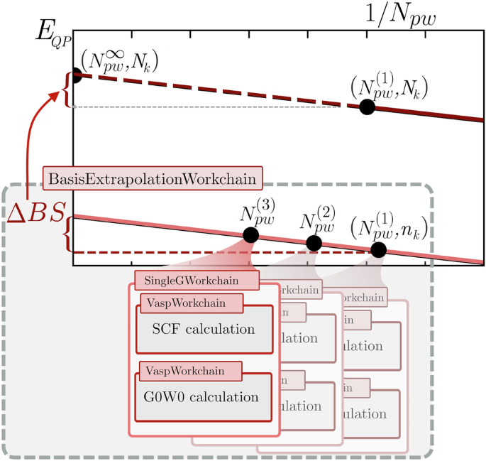
The higher-level BasisExtrWorkChain launches three instances of SingleGWorkChain to compute the QP energies on the low k-point density (nk) for the parameters \({N}_{pw}^{(1)},{N}_{pw}^{(2)}\) and \({N}_{pw}^{(3)}\). The asymptotic limit is extrapolated and the correction ΔBS, which is the main output of the BasisExtrWorkChain is determined and returned. Finally, the QP-energies on the dense k-point grid Nk are corrected on dense k-point grid (Nk).
The main VaspGWorkChain may call a second BasisExtrWorkChain instance and pass the NC-PAWs as inputs in order to compute \({E}_{QP\,\text{-}\,\infty }^{NC}({N}_{pw}^{\infty },{n}_{k})\) and the corresponding NV corrections. By default, this correction is skipped unless the structure contains elements whose US-PAWs exhibit non-negligible norm violations (the threshold is defined at 20% for the d partial-waves). The choice is performed automatically at runtime.
-
QP eigenvalues on the converged (dense) k-point mesh \({E}_{n{\bf{k}}}({N}_{pw}^{(1)},{N}_{k})\): SingleGWorkChain. This sub-workflow is an abstraction layer representing a complete G0W0 run. The workflow defines the logic needed to compute the QP energies for a specific structure, k-point mesh, and a specific number of bands and cutoff. It executes internally two different ab-initio simulations, the actual G0W0 calculation and the starting point DFT simulation, and returns the corresponding QP eigenvalues. A single SingleGWorkChain is launched to determine the QP energies \({E}_{QP}^{US}({N}_{pw},{N}_{k})\), on the dense k-mesh with US-PAW potentials. The Npw, \({G}_{cut}^{pw}\) parameters are selected as the less computationally expensive pair employed within the BasisExtrWorkChain.
-
Wannier-interpolation: WannierWorkChain. As a last step, this workchain can be called to interpolate the obtained QP energies through a Wannierization procedure to generate a QP band-structure along high-symmetry k-point directions.

We note that the BasisExtrWorkChain and KptsConvWorkChain both internally call SingleGWorkChain to perform the G0W0 runs. Furthermore, the lower level workflow is represented by VaspWorkchain, a core part of the AiiDA-VASP plugin which handles the actual ab-initio simulations on the remote high-performance clusters. It serves as a wrapper of a single generic VASP simulation and manages directly the construction of the VASP-specific files (INCAR, POSCAR, etc), the submission and the output parsing.
The modular structure is designed in such a way that BasisExtrWorkChain remains largely independent of the underlying ab-initio code and provides the general logic for computing the ΔBS and ΔNV corrections, while the SingleGWorkChain encapsulates VASP-specific logic and integrates directly with AiiDA-VASP workflows.
Besides the structural data, which represents the only mandatory inputs, the workchain accepts several other optional input parameters, which allow the user to override the default behavior of the workchain.
-
Deactivate_NVcorrection: Disable the NV correction.
-
Extrapolation_r2_Threshold: Specify the minimum threshold on the r2 determination coefficients for the extrapolation fit; if the calculated r2 falls below this threshold, the workflow will run an additional G0W\({}_{0}({N}_{pw}^{(4)},{n}_{k})\) calculation.
-
Selected_Mode: Enforce a specific protocol for determining the corrections.
-
Selected_Kpoint_mesh: If this input is provided, the k-points convergence procedure is bypassed, and the provided k-mesh is utilized as the dense Nk mesh.
-
Kpts_convergence_threshold: threshold value used to determine k-point convergence; the default value is set to 50 meV.
-
Deactivate_Wannierization: Skip the last Wannier interpolation step, activated by default.
-
Kpts_Wannierization_spacing: upper limit on the k-point spacing of a uniform grid employed for the Wannierization procedure; following Vitale et al., the default is set to ρk = 0.2 Å−1.
In the following sections, the main sub-workflows and their algorithms will be discussed in detail, starting from the workflow computing the Basis-Set Incompleteness error.
Basis extrapolation workchain
The algorithm encoded in the workchain is based on Eq. (4), and aims to extrapolate \({E}_{QP\text{-}\infty }({N}_{pw}^{\infty },{n}_{k})\) and the correction \(\Delta BS={E}_{QP\text{-}\infty }({N}_{pw}^{\infty },{n}_{k})-{E}_{QP}({N}_{pw}^{(1)},{n}_{k})\). We describe below its architecture:
-
Three G0W0 calculations are performed in parallel with different plane-wave cutoffs and band numbers, denoted respectively as \({{G}_{cut}^{pw}}^{(1)},{{G}_{cut}^{pw}}^{(2)},{{G}_{cut}^{pw}}^{(3)}\) and \({N}_{pw}^{(1)},{N}_{pw}^{(2)}\) and \({N}_{pw}^{(3)}\).
-
The cutoff of the first G0W0 data point is determined as the maximum energy cutoff (ENMAX tag) given in the pseudo-potentials, labeled \({G}_{pw}^{PAW}\), i.e., \({G}_{pw}^{(1)}={G}_{pw}^{PAW}\). \({N}_{pw}^{(1)}\) is determined by the full basis-set constraint.
-
The parameters of the subsequent two G0W0 data points are chosen in order to progressively increase the number of bands in steps of \(0.20\times {N}_{pw}^{(1)}\), i.e., \({N}_{pw}^{(2)}=1.2\times {N}_{pw}^{(1)}\) and \({N}_{pw}^{(3)}=1.4\times {N}_{pw}^{(1)}\). The corresponding \({{G}_{cut}^{pw}}^{(2)},{{G}_{cut}^{pw}}^{(3)}\) are defined by the full basis-set constraint.
-
The workflow performs a first extrapolation to compute \({E}_{QP\,\text{-}\,\infty }^{US}({N}_{pw}^{\infty },{n}_{k})\) (or \({E}_{QP\,\text{-}\,\infty }^{NC}({N}_{pw}^{\infty },{n}_{k})\), depending on the PAWs used). If the R2 determination coefficients of the linear fits exceed a predefined threshold (with a default value of 0.85, adjustable by the user through the input parameter Extrapolation_r2_Threshold), the extrapolations are deemed accurate and the extrapolated EQP-∞ values are returned. In cases where the condition is not satisfied, an additional fourth G0W0 calculation is performed with \({N}_{pw}^{(4)}=1.6\times {N}_{pw}^{(1)}\) and the fits are updated using the new data points.
This protocol represents a computationally efficient alternative to the one introduced by ref. 64, where the G0W0 calculations were performed employing a considerably larger number of bands, up to \({N}_{pw}^{(3)} \sim 2.0\times {N}_{pw}^{PAW}\). This choice is adopted as the default scheme. However, the application of this protocol to larger cells or supercells can be computationally demanding, as large cells are typically associated with a denser bandstructure which can potentially greatly increase the number of bands that need to be considered for the same Gcut. Therefore, we have introduced an alternative memory-conserving variant, which is suited for rapid screenings or for materials with large cells.
In the memory-conserving scheme, three separate calculations with \({{G}_{cut}^{pw}}^{(1)},{{G}_{cut}^{pw}}^{(2)},{{G}_{cut}^{pw}}^{(3)}\) defined by \(0.75\times {G}_{pw}^{PAW},1.00\times {G}_{pw}^{PAW},1.25\times {G}_{pw}^{PAW}\) are used for the extrapolation. The memory variant is active (default choice) for volumes larger than 150 Å3.
K-point convergence workchain
The KptsConvWorkChain finds the minimally dense k-point mesh which achieves convergence of the QP direct and indirect gaps within a given convergence tolerance. The search is restricted to uniform k-point meshes which include the high-symmetry k-points of the irreducible Brillouin Zone. To maintain computational efficiency, the workflow leverages the decoupling between the convergences of basis-set dimension and the k-point mesh density: the G0W0 calculations used to determine the converged k-point mesh are performed with a fixed and reduced basis-set dimension defined by \({G}_{cut}^{pw-kptsConv}=0.70\times {G}_{pw}^{PAW}\); the corresponding Npw is determined by the full basis-set constraint. The initial k-point mesh is selected based on a reciprocal-space resolution of 0.4 Å−1 along each lattice direction.
When the Wannierization procedure is enabled, an additional constraint must be taken into account: as outlined by Vitale et al.75, the automated Wannierization procedure requires a single input parameter, namely the k-point spacing of the uniform grid employed for the Wannierization procedure. Their work demonstrated how this parameter significantly impacts the accuracy of the resulting Wannier-interpolated band structure, and noted how a spacing of \({\rho }_{{\bf{k}}\text{-}\min }=0.2\) Å−1 is sufficient for achieving interpolations with errors less than 20 meV. This consideration is incorporated as an additional constraint on the convergence procedure. The minimum k-point spacing for the Wannier interpolation is taken by the workchain as an optional argument; the k-point meshes considered during the search are restricted to grids with a spacing equal to or higher than \({\rho }_{{\bf{k}}\text{-}\min }\).
Wannierization workchain
The interpolation of the GW band structure through an automatic Wannierization is performed by the WannierWorkChain sub-workflow. The starting projections are automatically determined using the selected columns of the density matrix (SCDM)100,101.
This sub-workchain executes a VASP simulation (via the VaspWorkchain) with Wannier90102 and its VASP interface87 starting from the wavefunctions on the dense k-point mesh Nk determined in the previous steps. An example of Wannierization obtained from this workflow is displayed in Fig. 4.

The G0W0 band structure of cubic SrTiO3 is automatically wannierized through the SCDM scheme and plotted alongside the G0W0 eigenvalues.
Validation against ab-initio references
This section is dedicated to the validation of the protocol implemented in the computational workflow: the main goal is to verify that the application of the NV and BS corrections can reliably reproduce the target quasi-particle energies \({E}_{QP-\infty }^{NC}({N}_{pw}^{\infty },{N}_{k})\). For this purpose, a reference dataset comprising the basis-set extrapolated \({E}_{QP-\infty }^{NC}({N}_{pw}^{\infty },{N}_{k})\) for 19 typical59,86,103,104 group III-VI semiconductors and insulators were determined through a careful extrapolation performed directly on the dense Nk grid (thus without the need of ΔBS and ΔNV). The results of the automated workflow for the same dataset are benchmarked against these reference \({E}_{QP-\infty }^{NC}\), and the differences (with and without the inclusion of the corrections) are compiled in Table 1 for valence band minimum (VBM) and conduction band maximum (CBM) at the Γ k-point. The complete QP energies for the considered set are compiled in Tables S3 and S4 in the SM. The inclusion of both corrections inside the workflow achieves a remarkable agreement with the reference QP energies, exhibiting a mean absolute error (MAE) of ~15 meV for the VBM and less than 10 meV for the CBM; this represents a sizeable error reduction compared to the data without the corrections, associated to MAEs of ~ 200 meV; the basis-set corrections alone account for the 45−50% of the error reductions for the considered dataset. However, the QP energies on US-PAW potentials \({E}_{QP}^{US}({N}_{pw}^{(1)})+\Delta BS\) still display a residual underestimation, in particular for group V and VI compounds (with ZnTe, MgO, InAs, GaAs and AlAs at ~−150 meV average) and markedly high for the ZnSe and CdSe VBMs. The inclusion of the NV correction successfully improves over the remaining errors, reducing the deviation from the reference \({E}_{QP-\infty }^{NC}\) to an average of under 20 meV. The proposed protocol is therefore able to reproduce the highly precise reference results with a reduced computational cost and without need of direct user interventions.
The G0W0 database
The workflow has been used to generate a database of QP gaps and energies comprising 325 distinct bulk structures. This database stands out, to the best of our knowledge, as one of the largest G0W0 datasets for bulk compounds available. It encompasses ~220 binary and ~100 ternary compounds, covering a gap range from 0.7 eV to 14 eV and containing ~ 40 diverse space groups (see Fig. 5a) for a distribution of the most represented spacegroup in the database). The full list of materials, including the predicted G0W0 gaps, the ΔBS and ΔNV corrections, is given in Table S5 in the SM. This expanded dataset enables a comprehensive evaluation of the accuracy of the predicted results, specifically assessing the performance of NV and BS corrections against experimental references (which were identified for 163 systems) and comparing them with prior G0W0 literature data.

a Distribution of compounds across the twenty most populated space-groups in the database. b Histogram showing the distribution of r2 determination coefficients for the extrapolations performed for the basis-set correction ΔBS using the default r2 threshold value, for the valence band maximum and conduction band minimum. c Violin plots of the percentage errors with respect to experiments for the entire G0W0 database and for the two subsets comprising all TM compounds and perovskite systems. The MAPEs and their corresponding standard deviations for each dataset are displayed within the boxes. d For each element the MAPE across all compounds containing that element (relative to experimental bandgaps) is displayed. The average Basis-Set (BS) and Norm-Violation (NV) corrections for each element are also included (shown only for values exceeding 0.03 eV for clarity). e Comparison between experimental and extrapolated G0W0 bandgaps; the TM points are highlighted in a different color. The shaded area and the dashed lines identify regions where errors are below 10% and 20%, respectively.
In order to ensure consistency with previous works47,64, we adopt a Γ-centered 6 × 6 × 6 grid as the dense k-point mesh Nk for the database. This grid choice has been established as converged up to around ~50 meV for insulators51,78,86,105 including binary transition metal oxides58,64,106,107,108,109,110,111,112,113,114,115, halides112,116, ternary TMOs and perovskites47,117. For materials displaying slow k-point convergence, like the TM oxide ZnO, the selected grid results in errors on the order of 100 meV64,65.
Two additional subsets have been integrated into the database to serve as additional test cases for further assessing the workflow’s efficacy. The first comprises 36 TM oxide perovskites, a class of materials which has often been used as proving grounds to propose or compare different computational schemes77,79,89,118,119,120. Furthermore, the presence of stronger degrees of electronic correlation establishes these systems as challenging benchmarks for electronic structure schemes, as exemplified by the substantial discrepancies and variability observed among theoretical predictions (covering for example a range from 3.36 eV79 to 4.05 eV47 for SrTiO3 and from 3.18 eV79 to 3.7 eV121 for BaTiO3). The systems in the second subset were selected from compounds known in the literature to present significant challenges to GW methods, in terms of severe dependence on the number of orbitals or because they yielded inconsistent and contrasting results in previous G0W0 studies. The former category includes ZnO and TM halides, which are noted as extreme cases due to the exceptionally high number of states required (estimated at more than 4000 for ZnO62,63,67 and ~8000 and ~4000 for CuCl and AgCl respectively116). Similar computational demands are additionally recognized for the perovskites SrTiO3 and BaTiO3. The latter category encompasses TM oxides such as MnO and NiO, along with several other compounds that demonstrated significant errors in a previous G0W0 HT study51 (SnO2, SnSe2, RuS2, V2O5 and CaO). The comparisons for this dataset are summarized in Fig. 6. For all magnetically ordered materials included in the database, spin-polarized calculations were performed using the known ground-state magnetic ordering.

a Comparison of absolute relative errors with respect to experimental bandgaps for the benchmark set. This subset includes compounds exhibiting substantial dependencies on the number of bands or large errors in previous HT studies51,52,138. The G0W0 gaps determined via the BS and NV corrections are depicted in red, alongside results from other HT studies (black)51,52,138, and G0W0@PBE values from references22,47,59,63,65,66,77,79,80,104,112,112,113,114,117,121,130,132,133,139,140,141,142,143,144,145,146,147,148,149,150,151,152,153,154,155,156,157,158,159,160,161,162,163,164,165,166 (blue). b Number of bands \({N}_{pw}^{(1)}\) included in the calculation on the dense k-mesh. c Values of the Basis-Set and Norm-Violation corrections.
Before discussing the workflow’s accuracy, we briefly examine the robustness of the extrapolation. The protocol relies on the assumption that the QP energies used to evaluate the corrections follow the 1 over Npw limit; to assess the validity of this hypothesis, the workflow automatically computes the r2 determination coefficients. The final r2 distributions (considering all materials in the database) for the Valence Band Maximum (VBM) and Conduction Band Minimum (CBM) are characterized by an average of respectively ~97% and ~ 96%, with a standard deviation of ~10% and ~12% (see Fig. 5b) for the histograms of the distributions). To further validate this approach, we tested a stricter threshold of r2 = 0.95 (defined via the input parameter Extrapolation_r2_Threshold) which prompts the workflow to perform an additional G0W0 calculations for materials with initial coefficient of determination 0.85 <= r2 < = 0.95.This additional calculation is then utilized in the extrapolation for the BS correction (see Fig. S4 in the SI). This adaptive approach successfully improved the extrapolation accuracy, demonstrating the reliability of the protocol.
Validation against experimental references
A graphical summary of the errors with respect to the experimental references over the entire dataset is presented in Fig. 5: Fig. 5c) represents a violin plot of the percentage errors for the entire database and for the TM and perovskite, subsets, Fig. 5e) shows a scatter plot of the extrapolated G0W0 gaps against the experimental ones, while the distributions of the mean absolute percentage errors over the materials containing the given element is shown in Fig. 5d), along with the average BS and NV corrections. The workflow is able to achieve a mean absolute percentage error (MAPE) of ~6.7% (see Table 2), corresponding to state-of-the-art accuracy. This value is reached, including all 163 systems with experimental references, representing a robust and comprehensive evaluation of the workflow performance. Only a minority fraction, comprising 22 materials, shows errors exceeding 10%: the outliers include chalcogenides (BeS, SnSe2, WSe2 and TlSe), as well as cuprates (Cu2O and CuCl) and heavy 4-d and 5-d compounds (Bi2Te3, BiOCl, PbF2 and HfO2). The larger discrepancies identified above for the heavy 4-d and 5-d compounds122,123,124 can be explained by the omission of the spin-orbit coupling (SOC), which is known to result in significant errors, up to 0.3–0.4 eV98,125,126. Additionally, electron-phonon coupling can also affect predicted band gaps. Several studies demonstrated how zero-point renormalization (ZPR) can lead to reduction of the gap by ~0.15–0.20 eV for several systems present in the dataset, including BaSnO3, SnO2 or ZnO103,127,128. In addition, as noted in the Methods section, deviations from experimental values may also arise from the lack of self-consistency in the energy and screened interaction W, as well as from the omission of vertex corrections. These factors that are particularly important for excitonic materials and transition metal oxides88,89.
We must also note that the heterogeneity of temperatures, quality of the samples (e.g., degree of crystallinity, defects, etc.) and experimental techniques employed in the reference measurements introduce non-controllable uncertainties in the comparison with our data.
For systems without transition metals, the workflow achieves an MAPE around 5.5%. Conversely, transition metal compounds are recognized as some of the more critical and demanding cases for G0W0@DFT, as evidenced by higher deviations from the experimental data (with a MAPE of 8.6%). The description of the localized partially filled d states presents several difficulties, beginning from using DFT as a starting point32,129,130. In particular, the requirements on the number of states for the self-energy and the norm violations associated with TM PAWs are typically exacerbated, potentially evolving into critical issues for such materials32,47,64. For example, the 3-d US-PAWs exhibit the largest norm violations among the entire dataset, ranging from ~25% for the d partial-waves of Ti and V up to ~57% for Cu. These two factors explain the higher on average NV and BS corrections for TM systems observed in Fig. 5d), which reach the maximum for the strongly localized 3-d states or 2-p states131 (as in the case of fluorine). In fact, the higher ΔBS and ΔNV correct the larger basis-set truncation errors on the energies \({E}_{QP}^{US}\) involving localized states In line with these considerations, compounds containing Cu are associated with the highest values of ΔNV and ΔBS among the database, with the halides displaying ΔBS ~ 0.20 eV and ΔNV ~ 0.50 eV, respectively).
The inclusion of ΔNV and ΔBS is notably accurate for all transition metal compounds in the second subset: as shown in Fig. 6, the protocol consistently reproduces or slightly improves over the most accurate G0W0@DFT results reported in the literature for nearly all these materials. Furthermore, the workflow proves effective also for the perovskite subset, achieving a MAPE of ~5.6% associated with a similar MAE of 0.20 eV.
Importantly, the workflow design enables an efficient computational setup. The protocol requires only a fixed number of 3-4 G0W0 calculations for basis-set extrapolation (or 6-8 when norm-violation correction is applied), making this approach highly competitive compared to high-throughput protocols that rely on explicit exploration of the \(({N}_{pw},{G}_{cut}^{pw})\) parameter space; for instance, a recent benchmark54 on a dataset of 60 bulk materials has shown that such parameter-space exploration algorithms typically require a mean of between 7 and 14 GW computations per material (depending on the specifics of the algorithm used).
Secondly, the G0W0 calculation on the dense k-point mesh \({E}_{QP}^{US}({N}_{pw}^{(1)},{N}_{k})\) —typically the most computationally expensive step (see SM Fig. S1)—can be performed with substantially reduced computational requirements by employing US-PAW potentials, which impose significantly lower cutoffs and Npw (see SM Fig. S2). In turn the ΔNV corrections restore the accuracy of norm-conserving PAWs’ results. This approach proves particularly valuable for TM compounds, which often require NC potentials with very high cutoffs and Npw. The protocol achieves substantial computational savings for nearly all TM systems in Fig. 6, reducing band requirements to at most half those referenced in the literature without compromising accuracy, requiring at most 1000 bands and cutoffs \({G}_{cut}^{pw}\) up to ~450 eV to compute \({E}_{QP}^{US}({N}_{pw}^{(1)},{N}_{k})\). In particular, the TM oxide ZnO and the copper halides (which as mentioned poses remarkably high Npw convergence requirements and also exhibited the largest errors in previous HT G0W0 study51)—necessitate approximately \({N}_{pw}^{(1)} \sim 1200\) bands.
The previously cited perovskites SrTiO3 and BaTiO3 exhibit similar convergence criticalities, with different studies based on conventional convergence procedures reporting convergence requirements between 2000 and 5000 bands47,132; our workflow in turn achieves state-of-the-art accuracy with ~1000 bands (and ~440 eV of \({G}_{cut}^{pw}\) cutoff), due to ΔBS and ΔNV around ~0.20 eV. Lastly, we note that the protocol requires a larger number of bands for layered oxide V2O5 (~2300), due to the larger volume of the unit cell. Nonetheless, our setup employed a cutoff ~ 440 eV to determine QP energies on the dense Nk mesh for V2O5, a comparably lower value with respect to the ~1100–1400 eV demanded by recent GW and QSGW studies133,134,135. A runtime comparison between US and NC potentials for these selected systems is provided in Figure S1 of the Supporting Information.
Discussion
In this work, we have presented the development and validation of a high-throughput automatized approach for computing G0W0 quasi-particle energies using the AiiDA-VASP framework. The approach is based on the estimation and correction of errors related to the basis-set truncation and PAW norm violation. To showcase its effectiveness and for benchmark purposes, a comprehensive database encompassing 325 materials was constructed using the proposed workflow. From a theoretical point of view, the correction scheme respects the full basis-set constraint, which formally ensures the correct asymptotic limit. An extensive validation, performed involving more than 160 different systems, shows that the automated procedure is able to achieve state-of-the-art accuracy while requiring minimal user intervention. The workflow’s computational efficiency represents a second important advantage of the protocol. The scheme does not need to sample multidimensional parameter spaces, strongly limiting the total number of calculations required. Further developments of the workflow, aimed at improving accuracy for critical cases, could involve integrating ZPR as well as the additional contributions due to vertex corrections and SOC. The presented results illustrate how the proposed workflow, which requires only the structural data, can represent a powerful resource for the material science community for high-throughput excited-state studies with high accuracy. Finally, the complete database collected in the supplementary data offers a valuable reference for future studies, facilitating comparison and benchmarking across ab-initio codes.
Methods
General computational setup for ab-initio calculations
All calculations are performed using Vienna Ab-initio Simulation Package (VASP)68,69, version 6.2.0. The GW versions of the US-PAW pseudo-potentials136,137, with relativistic effects taken into account only at scalar level and semicore electrons included (where available), are selected for all elements. The complete list of the US-PAWs and NC-PAWs is listed in SM (see Tables SM1 and SM2). The table also lists the maximum norm violation among the pseudo-waves for each PAW potential. Unless explicitly stated, the ultra-soft PAW (non norm-conserving) version of the pseudo-potentials is chosen.
Computational details for G0W0 calculations
All results discussed in the text are obtained using the quartic-scaling G0W0 scheme, using DFT (PBE) as a starting point. The Spin-Orbit effects are not taken into account. The full frequency dependent self-energy is evaluated through the Hilbert transform technique78 including 200 frequency points. Furthermore, all G0W0 results presented include the settings PREC = Accurate, which forces VASP to employ a denser than standard FFT grid. The NMAXFOCKAE flag, which controls the cutoff used for the reconstruction for the overlap densities in the PAW scheme, is set equal to NMAXFOCKAE =2. The Wannierization is performed with the Wannier90 code102m version 3.1, which is called inside the VASP calculations in library mode.
Data availability
The dataset composing the G0W0 database will be made publicly available and accessible; the NC-PAW potentials will be released in the next version of the VASP software.
Code availability
The source code is available open-source on GitHub (https://github.com/orgs/QuantumMaterialsModelling/ or https://github.com/lorenzovarro/GW-VASP-workflow) and will be part of the next release of the AiiDA-VASP plugin.
References
Curtarolo, S. et al. The high-throughput highway to computational materials design. Nat. Mater. 12, 191–201 (2013).
Thygesen, K. S. & Jacobsen, K. W. Making the most of materials computations. Science 354, 180–181 (2016).
Alberi, K. et al. The 2019 materials by design roadmap. J. Phys. D Appl. Phys. 52, 013001 (2018).
Schaarschmidt, J. et al. Workflow engineering in materials design within the BATTERY 2030+ project. Adv. Energy Mater. 12, 2102638 (2022).
Jain, A. et al. FireWorks: a dynamic workflow system designed for high-throughput applications. Concurrency Comput. Pract. Exp.27, 5037–5059 (2015).
Pizzi, G., Cepellotti, A., Sabatini, R., Marzari, N. & Kozinsky, B. AiiDA: automated interactive infrastructure and database for computational science. Comput. Mater. Sci. 111, 218–230 (2016).
Mortensen, J. J., Gjerding, M. & Thygesen, K. S. MyQueue: Task and workflow scheduling system. J. Open Source Softw. 5, 1844 (2020).
Curtarolo, S. et al. AFLOW: An automatic framework for high-throughput materials discovery. Comput. Mater. Sci. 58, 218–226 (2012).
Mathew, K. et al. Atomate: A high-level interface to generate, execute, and analyze computational materials science workflows. Comput. Mater. Sci. 139, 140–152 (2017).
Kirklin, S. et al. The open quantum materials database (oqmd): assessing the accuracy of DFT formation energies. npj Comput. Mater. 1, 15010 (2015).
Jain, A. et al. Commentary: The Materials Project: A materials genome approach to accelerating materials innovation. APL Mater. 1, https://doi.org/10.1063/1.4812323 (2013).
Draxl, C. & Scheffler, M. The nomad laboratory: from data sharing to artificial intelligence. J. Phys. Mater. 2, 036001 (2019).
Mounet, N. et al. Two-dimensional materials from high-throughput computational exfoliation of experimentally known compounds. Nat. Nanotechnol. 13, 246–252 (2018).
Talirz, L. et al. Materials Cloud, a platform for open computational science. Sci. Data 7, 299 (2020).
Schmidt, J., Marques, M. R. G., Botti, S. & Marques, M. A. L. Recent advances and applications of machine learning in solid-state materials science. npj Comput. Mater. 5, 83 (2019).
Wang, A. Y.-T. et al. Machine learning for materials scientists: an introductory guide toward best practices. Chem. Mater. 32, 4954–4965 (2020).
Ashton, M., Paul, J., Sinnott, S. B. & Hennig, R. G. Topology-scaling identification of layered solids and stable exfoliated 2D materials. Phys. Rev. Lett. 118, 106101 (2017).
Cheon, G. et al. Data mining for new two- and one-dimensional weakly bonded solids and lattice-commensurate heterostructures. Nano Lett. 17, 1915–1923 (2017).
Huber, S. P. et al. Common workflows for computing material properties using different quantum engines. npj Comput. Mater. 7, 136 (2021).
Bosoni, E. et al. How to verify the precision of density-functional-theory implementations via reproducible and universal workflows. Nat. Rev. Phys. 6, 45–58 (2024).
Carbogno, C. et al. Numerical quality control for DFT-based materials databases. npj Comput. Mater. 8, 69 (2022).
Rasmussen, F. A. & Thygesen, K. S. Computational 2D materials database: electronic structure of transition-metal dichalcogenides and oxides. J. Phys. Chem. C. 119, 13169–13183 (2015).
Choudhary, K., Kalish, I., Beams, R. & Tavazza, F. High-throughput identification and characterization of two-dimensional materials using density functional theory. Sci. Rep. 7, 5179 (2017).
Kirklin, S., Meredig, B. & Wolverton, C. High-throughput computational screening of new Li-ion battery anode materials. Adv. Energy Mater. 3, 252–262 (2013).
Bhattacharya, S. & Madsen, G. K. H. High-throughput exploration of alloying as design strategy for thermoelectrics. Phys. Rev. B 92, 085205 (2015).
Hautier, G., Miglio, A., Ceder, G., Rignanese, G.-M. & Gonze, X. Identification and design principles of low hole effective mass p-type transparent conducting oxides. Nat. Commun. 4, 2292 (2013).
Chen, W. et al. Understanding thermoelectric properties from high-throughput calculations: trends, insights, and comparisons with experiment. J. Mater. Chem. C. 4, 4414–4426 (2016).
Marrazzo, A., Gibertini, M., Campi, D., Mounet, N. & Marzari, N. Relative abundance of z2 topological order in exfoliable two-dimensional insulators. Nano Lett. 19, 8431–8440 (2019).
Zhang, Z. et al. Computational screening of layered materials for multivalent ion batteries. ACS Omega 4, 7822–7828 (2019).
Kahle, L., Marcolongo, A. & Marzari, N. High-throughput computational screening for solid-state Li-ion conductors. Energy Environ. Sci. 13, 928–948 (2020).
Godby, R. W., Schlüter, M. & Sham, L. J. Accurate exchange-correlation potential for silicon and its discontinuity on addition of an electron. Phys. Rev. Lett. 56, 2415–2418 (1986).
Golze, D., Dvorak, M. & Rinke, P. The GW Compendium: a practical guide to theoretical photoemission spectroscopy. Front. Chem. 7 (2019).
Onida, G., Reining, L. & Rubio, A. Electronic excitations: density-functional versus many-body green’s-function approaches. Rev. Mod. Phys. 74, 601–659 (2002).
Hachmann, J. et al. The Harvard Clean Energy Project: large-scale computational screening and design of organic photovoltaics on the world community grid. J. Phys. Chem. Lett. 2, 2241–2251 (2011).
He, Q., Yu, B., Li, Z. & Zhao, Y. Density functional theory for battery materials. Energy Environ. Mater. 2, 264–279 (2019).
Lee, M., Youn, Y., Yim, K. & Han, S. High-throughput ab initio calculations on dielectric constant and band gap of non-oxide dielectrics. Sci. Rep. 8, 14794 (2018).
Dudarev, S. L., Botton, G. A., Savrasov, S. Y., Humphreys, C. J. & Sutton, A. P. Electron-energy-loss spectra and the structural stability of nickel oxide: an lsda+u study. Phys. Rev. B 57, 1505–1509 (1998).
Krukau, A. V., Vydrov, O. A., Izmaylov, A. F. & Scuseria, G. E. Influence of the exchange screening parameter on the performance of screened hybrid functionals. J. Chem. Phys. 125, 224106 (2006).
Yan, Q. et al. Solar fuels photoanode materials discovery by integrating high-throughput theory and experiment. Proc. Natl Acad. Sci. 114, 3040–3043 (2017).
Xiong, Y. et al. Optimizing accuracy and efficacy in data-driven materials discovery for the solar production of hydrogen. Energy Environ. Sci. 14, 2335–2348 (2021).
Kim, S. et al. A band-gap database for semiconducting inorganic materials calculated with hybrid functional. Sci. Data 7, 387 (2020).
Hinuma, Y., Kumagai, Y., Tanaka, I. & Oba, F. Band alignment of semiconductors and insulators using dielectric-dependent hybrid functionals: Toward high-throughput evaluation. Phys. Rev. B 95, 075302 (2017).
Liu, M., Gopakumar, A., Hegde, V. I., He, J. & Wolverton, C. High-throughput hybrid-functional DFT calculations of bandgaps and formation energies and multifidelity learning with uncertainty quantification. Phys. Rev. Mater. Accepted for publication (2024).
Castelli, I. E. et al. Computational screening of perovskite metal oxides for optimal solar light capture. Energy Environ. Sci. 5, 5814–5819 (2012).
Kuhar, K., Pandey, M., Thygesen, K. S. & Jacobsen, K. W. High-Throughput computational assessment of previously synthesized semiconductors for photovoltaic and photoelectrochemical devices. ACS Energy Lett. 3, 436–446 (2018).
Van Setten, M. J., Popa, V. A., De Wijs, G. A. & Brocks, G. Electronic structure and optical properties of lightweight metal hydrides. Phys. Rev. B Condens. Matter Mater. Phys. 75, 035204 (2007).
Ergönenc, Z., Kim, B., Liu, P., Kresse, G. & Franchini, C. Converged GW quasiparticle energies for transition metal oxide perovskites. Phys. Rev. Mater. 2 (2018).
Haastrup, S. et al. The computational 2d materials database: high-throughput modeling and discovery of atomically thin crystals. 2D Mater. 5, 042002 (2018).
Rasmussen, A., Deilmann, T. & Thygesen, K. S. Towards fully automated GW band structure calculations: What we can learn from 60.000 self-energy evaluations. npj Comput. Mater. 7, 22 (2021).
Lee, J., Seko, A., Shitara, K., Nakayama, K. & Tanaka, I. Prediction model of band gap for inorganic compounds by combination of density functional theory calculations and machine learning techniques. Phys. Rev. B 93, 115104 (2016).
van Setten, M. J., Giantomassi, M., Gonze, X., Rignanese, G.-M. & Hautier, G. Automation methodologies and large-scale validation for GW: Towards high-throughput GW calculations. Phys. Rev. B 96, 155207 (2017).
Bonacci, M. et al. Towards high-throughput many-body perturbation theory: efficient algorithms and automated workflows. npj Comput. Mater. 9, 74 (2023).
Biswas, T. & Singh, A. K. pyGWBSE: a high throughput workflow package for GW-BSE calculations. npj Comput. Mater. 9, 22 (2023).
Großmann, M., Grunert, M. & Runge, E. A robust, simple, and efficient convergence workflow for GW calculations. npj Comput. Mater. 10, 135 (2024).
Hedin, L. New method for calculating the one-particle Green’s function with application to the electron-gas problem. Phys. Rev. 139, A796–A823 (1965).
Strinati, G., Mattausch, H. J. & Hanke, W. Dynamical aspects of correlation corrections in a covalent crystal. Phys. Rev. B 25, 2867–2888 (1982).
Reining, L. The GW approximation: content, successes and limitations. WIREs Comput. Mol. Sci. 8, e1344 (2018).
Shishkin, M. & Kresse, G. Self-consistent GW calculations for semiconductors and insulators. Phys. Rev. B 75, 235102 (2007).
van Schilfgaarde, M., Kotani, T. & Faleev, S. Quasiparticle self-consistent gw theory. Phys. Rev. Lett. 96, 226402 (2006).
van Setten, M. J. et al. GW100: Benchmarking G0W0 for molecular systems. J. Chem. Theory Comput. 11, 5665–5687 (2015).
Knight, J. W. et al. Accurate ionization potentials and electron affinities of acceptor molecules III: A benchmark of GW methods. J. Chem. Theory Comput. 12, 615–626 (2016).
Shih, B.-C., Xue, Y., Zhang, P., Cohen, M. L. & Louie, S. G. Quasiparticle band gap of ZnO: High accuracy from the conventional G0W0 approach. Phys. Rev. Lett. 105, 146401 (2010).
Friedrich, C., Müller, M. C. & Blügel, S. Band convergence and linearization error correction of all-electron GW calculations: the extreme case of zinc oxide. Phys. Rev. B 83, 081101 (2011).
Klimeš, Jcv, Kaltak, M. & Kresse, G. Predictive GW calculations using plane waves and pseudopotentials. Phys. Rev. B 90, 075125 (2014).
Stankovski, M. et al. G0W0 band gap of ZnO: effects of plasmon-pole models. Phys. Rev. B 84, 241201 (2011).
Gao, W., Xia, W., Gao, X. & Zhang, P. Speeding up GW calculations to meet the challenge of large-scale Quasiparticle predictions. Sci. Rep. 6, 36849 (2016).
Rangel, T. et al. Reproducibility in G0W0 calculations for solids. Comput. Phys. Commun. 255, 107242 (2020).
Kresse, G. & Furthmüller, J. Efficient iterative schemes for ab initio total-energy calculations using a plane-wave basis set. Phys. Rev. B Condens. Matter Mater. Phys. 54, 11169–11186 (1996).
Kresse, G. & Furthmüller, J. Efficiency of ab-initio total energy calculations for metals and semiconductors using a plane-wave basis set. Comput. Mater. Sci. 6, 15–50 (1996).
Blöchl, P. E. Projector augmented-wave method. Phys. Rev. B 50, 17953–17979 (1994).
Uhrin, M., Huber, S. P., Yu, J., Marzari, N. & Pizzi, G. Workflows in AiiDA: engineering a high-throughput, event-based engine for robust and modular computational workflows. Comput. Mater. Sci. 187, 110086 (2021).
Prandini, G., Marrazzo, A., Castelli, I. E., Mounet, N. & Marzari, N. Precision and efficiency in solid-state pseudopotential calculations. npj Comput. Mater. 4, 72 (2018).
Mercado, R. et al. In silico design of 2D and 3D covalent organic frameworks for Methane storage applications. Chem. Mater. 30, 5069–5086 (2018).
Atambo, M. O. et al. Electronic and optical properties of doped Tio2 by many-body perturbation theory. Phys. Rev. Mater. 3, 045401 (2019).
Vitale, V. et al. Automated high-throughput Wannierisation. npj Comput. Mater. 6, 66 (2020).
Lebègue, S., Arnaud, B., Alouani, M. & Bloechl, P. E. Implementation of an all-electron gw approximation based on the projector augmented wave method without plasmon pole approximation: application to Si, SiC, AlAs, InAs, NaH, and KH. Phys. Rev. B 67, 155208 (2003).
van Schilfgaarde, M., Kotani, T. & Faleev, S. V. Adequacy of approximations in GW theory. Phys. Rev. B 74, 245125 (2006).
Shishkin, M. & Kresse, G. Implementation and performance of the frequency-dependent GW method within the paw framework. Phys. Rev. B 74, Arnaud (2006).
Friedrich, C., Blügel, S. & Schindlmayr, A. Efficient implementation of the GW approximation within the all-electron FLAPW method. Phys. Rev. B 81, 125102 (2010).
Kotani, T. & van Schilfgaarde, M. All-electron GW approximation with the mixed basis expansion based on the full-potential LMTO method. Solid State Commun. 121, 461–465 (2002).
Rinke, P., Qteish, A., Neugebauer, J., Freysoldt, C. & Scheffler, M. Combining GW calculations with exact-exchange density-functional theory: an analysis of valence-band photoemission for compound semiconductors. N. J. Phys. 7, 126 (2005).
Faleev, S. V., van Schilfgaarde, M. & Kotani, T. All-electron self-consistent GW approximation: application to Si, MnO, and NiO. Phys. Rev. Lett. 93, 126406 (2004).
Kotani, T., van Schilfgaarde, M. & Faleev, S. V. Quasiparticle self-consistent GW method: a basis for the independent-particle approximation. Phys. Rev. B 76, 165106 (2007).
Reining, L., Olevano, V., Rubio, A. & Onida, G. Excitonic effects in solids described by time-dependent density-functional theory. Phys. Rev. Lett. 88, 066404 (2002).
Adragna, G., Del Sole, R. & Marini, A. Ab initio calculation of the exchange-correlation kernel in extended systems. Phys. Rev. B 68, 165108 (2003).
Shishkin, M., Marsman, M. & Kresse, G. Accurate quasiparticle spectra from self-consistent GW calculations with vertex corrections. Phys. Rev. Lett. 99, 246403 (2007).
Franchini, C. et al. Maximally localized wannier functions in lamno3 within pbe + u, hybrid functionals and partially self-consistent gw: an efficient route to construct ab initio tight-binding parameters for eg perovskites. J. Phys. Condens. Matter 24, 235602 (2012).
Cunningham, B., Grüning, M., Pashov, D. & van Schilfgaarde, M. QS GW: quasiparticle self-consistent GW with ladder diagrams in w. Phys. Rev. B 108, 165104 (2023).
Varrassi, L., Liu, P. & Franchini, C. Quasiparticle and excitonic properties of monolayer srtio3. Phys. Rev. Mater. 8, 024001 (2024).
Aryasetiawan, F. & Gunnarsson, O. The GW method. Rep. Prog. Phys. 61, 237–312 (1998).
Harl, J. & Kresse, G. Cohesive energy curves for noble gas solids calculated by adiabatic connection fluctuation-dissipation theory. Phys. Rev. B 77, 045136 (2008).
Shepherd, J. J., Grüneis, A., Booth, G. H., Kresse, G. & Alavi, A. Convergence of many-body wave-function expansions using a plane-wave basis: From homogeneous electron gas to solid state systems. Phys. Rev. B 86, 035111 (2012).
Gulans, A. Towards numerically accurate many-body perturbation theory: short-range correlation effects. J. Chem. Phys. 141, 164127 (2014).
Schindlmayr, A. Analytic evaluation of the electronic self-energy in the GW approximation for two electrons on a sphere. Phys. Rev. B 87, 075104 (2013).
Björkman, T., Gulans, A., Krasheninnikov, A. V. & Nieminen, R. M. van der Waals bonding in layered compounds from advanced density-functional first-principles calculations. Phys. Rev. Lett. 108, 235502 (2012).
Gonze, X. et al. The abinit project: Impact, environment and recent developments. Comput. Phys. Commun. 248, 107042 (2020).
Mortensen, J. J. et al. GPAW: an open Python package for electronic structure calculations. J. Chem. Phys. 160, 092503 (2024).
Grüneis, A., Kresse, G., Hinuma, Y. & Oba, F. Ionization potentials of solids: the importance of vertex corrections. Phys. Rev. Lett. 112, 096401 (2014).
AiiDA-VASP plugin page. https://github.com/aiida-vasp/aiida-vasp. Accessed: 22-06-2023.
Damle, A., Lin, L. & Ying, L. Compressed representation of Kohn-Sham orbitals via selected columns of the density matrix. J. Chem. Theory Comput. 11, 1463–1469 (2015).
Damle, A. & Lin, L. Disentanglement via entanglement: a unified method for Wannier localization. Multiscale Model. Simul. 16, 1392–1410 (2018).
Pizzi, G. et al. Wannier90 as a community code: new features and applications. J. Phys. Condens. Matter 32, 165902 (2020).
Miglio, A. et al. Predominance of non-adiabatic effects in zero-point renormalization of the electronic band gap. npj Comput. Mater. 6, 167 (2020).
Bhandari, C., van Schilfgaarde, M., Kotani, T. & Lambrecht, W. R. L. All-electron quasiparticle self-consistent GW band structures for SrTio3 including lattice polarization corrections in different phases. Phys. Rev. Mater. 2, 013807 (2018).
Gant, S. E. et al. Optimally tuned starting point for single-shot GW calculations of solids. Phys. Rev. Mater. 6, 053802 (2022).
Bhandari, C., Lambrecht, W. R. L. & van Schilfgaarde, M. Quasiparticle self-consistent gw calculations of the electronic band structure of bulk and monolayer v2o5. Phys. Rev. B 91, 125116 (2015).
Sklénard, B., Dragoni, A., Triozon, F. & Olevano, V. Optical vs electronic gap of hafnia by ab initio Bethe-Salpeter equation. Appl. Phys. Lett. 113, 172903 (2018).
Malashevich, A., Jain, M. & Louie, S. G. First-principles DFT+GW study of oxygen vacancies in rutile Tio2. Phys. Rev. B 89, 075205 (2014).
Patrick, C. E. & Giustino, F. Gw quasiparticle bandgaps of anatase tio2 starting from dft + u. J. Phys. Condens. Matter 24, 202201 (2012).
Jiang, H., Gomez-Abal, R. I., Rinke, P. & Scheffler, M. Electronic band structure of zirconia and hafnia polymorphs from the GW perspective. Phys. Rev. B 81, 085119 (2010).
Kang, W. & Hybertsen, M. S. Quasiparticle and optical properties of rutile and anatase tio2. Phys. Rev. B 82, 085203 (2010).
Chen, W. & Pasquarello, A. Accurate band gaps of extended systems via efficient vertex corrections in GW. Phys. Rev. B 92, 041115 (2015).
Jiang, H., Gomez-Abal, R. I., Rinke, P. & Scheffler, M. First-principles modeling of localized d states with the GW@LDA+u approach. Phys. Rev. B 82, 045108 (2010).
Das, S., Coulter, J. E. & Manousakis, E. Convergence of quasiparticle self-consistent GW calculations of transition-metal monoxides. Phys. Rev. B 91, 115105 (2015).
Jiang, H. Revisiting the GW approach to d- and f-electron oxides. Phys. Rev. B 97, 245132 (2018).
Gao, W. et al. Quasiparticle band structures of CuCl, CuBr, AgCl, and AgBr: the extreme case. Phys. Rev. B 98, 045108 (2018).
Gierlich, A. & Blügel, S. All-electron gw calculations for perovskite transition-metal oxides. Bull. Am. Phys. Soc. 2010 https://api.semanticscholar.org/CorpusID:94225183 (2010).
Varrassi, L. et al. Optical and excitonic properties of transition metal oxide perovskites by the Bethe-Salpeter equation. Phys. Rev. Mater. 5, 074601 (2021).
Tröster, A. et al. Hard antiphase domain boundaries in strontium titanate unravelled using machine-learned force fields. Phys. Rev. Mater. 6, 094408 (2022).
He, J. & Franchini, C. Screened hybrid functional applied to 3d0→3d8 transition-metal perovskites lamo3 (m = sc–cu): influence of the exchange mixing parameter on the structural, electronic, and magnetic properties. Phys. Rev. B 86, 235117 (2012).
Sanna, S., Thierfelder, C., Wippermann, S., Sinha, T. P. & Schmidt, W. G. Barium titanate ground- and excited-state properties from first-principles calculations. Phys. Rev. B 83, 054112 (2011).
Riley, J. M. et al. Direct observation of spin-polarized bulk bands in an inversion-symmetric semiconductor. Nat. Phys. 10, 835–839 (2014).
Ganose, A. M., Cuff, M., Butler, K. T., Walsh, A. & Scanlon, D. O. Interplay of orbital and relativistic effects in bismuth oxyhalides: BiOF, BiOCl, BiOBr, and BiOI. Chem. Mater. 28, 1980–1984 (2016).
Garcia, J. C. et al. Effective masses and complex dielectric function of cubic HfO2. Appl. Phys. Lett. 85, 5022–5024 (2004).
Kühn, M. & Weigend, F. One-electron energies from the two-component GW method. J. Chem. Theory Comput. 11, 969–979 (2015).
Scherpelz, P., Govoni, M., Hamada, I. & Galli, G. Implementation and validation of fully relativistic GW calculations: spin–orbit coupling in molecules, nanocrystals, and solids. J. Chem. Theory Comput. 12, 3523–3544 (2016).
Aggoune, W. et al. A consistent picture of excitations in cubic BaSnO3 revealed by combining theory and experiment. Commun. Mater. 3, 12 (2022).
Engel, M. et al. Zero-point renormalization of the band gap of semiconductors and insulators using the projector augmented wave method. Phys. Rev. B 106, 094316 (2022).
He, J. & Franchini, C. Structural determination and electronic properties of the 4d perovskite SrPDO3. Phys. Rev. B 89, 045104 (2014).
Liu, P., Franchini, C., Marsman, M. & Kresse, G. Assessing model-dielectric-dependent hybrid functionals on the antiferromagnetic transition-metal monoxides mno, feo, coo, and nio. J. Phys. Condens. Matter 32, 015502 (2019).
Maggio, E., Liu, P., van Setten, M. J. & Kresse, G. GW100: a plane wave perspective for small molecules. J. Chem. Theory Comput. 13, 635–648 (2017).
Lopez-Candales, G., Tang, Z., Xia, W., Jia, F. & Zhang, P. Quasiparticle band structure of SrTiO3 and BaTiO3: a combined LDA+u and G0W0 approach. Phys. Rev. B 103, 035128 (2021).
Gorelov, V., Reining, L., Lambrecht, W. R. L. & Gatti, M. Robustness of electronic screening effects in electron spectroscopies: example of v2o5. Phys. Rev. B 107, 075101 (2023).
Gorelov, V. et al. Delocalization of dark and bright excitons in flat-band materials and the optical properties of v2o5. npj Comput. Mater. 8, 94 (2022).
Roginskii, E. M. et al. A computational and spectroscopic study of the electronic structure of V2O5-based cathode materials. J. Phys. Chem. C 125, 5848–5858 (2021).
Perdew, J. P., Burke, K. & Ernzerhof, M. Generalized gradient approximation made simple. Phys. Rev. Lett. 77, 3865–3868 (1996).
Kresse, G. & Joubert, D. From ultrasoft pseudopotentials to the projector augmented-wave method. Phys. Rev. B Condens. Matter Mater. Phys. 59, 1758–1775 (1999).
Abedi, S. et al. A benchmark of first-principles methods for accurate prediction of semiconductor band gaps (2022).
Zhang, M.-Y. & Jiang, H. Electronic band structure of cuprous and silver halides: an all-electron GW study. Phys. Rev. B 100, 205123 (2019).
Abedi, S. et al. Statistical analysis of the performance of a variety of first-principles schemes for accurate prediction of binary semiconductor band gaps. J. Chem. Phys. 158, 184109 (2023).
Yeh, C.-N., Shee, A., Sun, Q., Gull, E. & Zgid, D. Relativistic self-consistent GW: exact two-component formalism with one-electron approximation for solids. Phys. Rev. B 106, 085121 (2022).
Choudhary, K. et al. Accelerated discovery of efficient solar cell materials using quantum and machine-learning methods. Chem. Mater. 31, 5900–5908 (2019).
Pishtshev, A. & Karazhanov, S. Z. Structure-property relationships in cubic cuprous iodide: a novel view on stability, chemical bonding, and electronic properties. J. Chem. Phys. 146, 064706 (2017).
Riefer, A. et al. Interplay of excitonic effects and van Hove singularities in optical spectra: Cao and Aln polymorphs. Phys. Rev. B 84, 075218 (2011).
Poncé, S. et al. First-principles and experimental characterization of the electronic and optical properties of cas and cao. Optical Mater. 35, 1477–1480 (2013).
Nejatipour, H. & Dadsetani, M. Excitonic effects in the optical properties of alkaline earth chalcogenides from first-principles calculations. Phys. Scr. 90, 085802 (2015).
Berger, J. A., Reining, L. & Sottile, F. Efficient GW calculations for SnO2, ZnO, and rubrene: the effective-energy technique. Phys. Rev. B 85, 085126 (2012).
Usuda, M., Hamada, N., Kotani, T. & van Schilfgaarde, M. All-electron GW calculation based on the LAPW method: application to wurtzite ZnO. Phys. Rev. B 66, 125101 (2002).
Miglio, A. et al. Effects of plasmon pole models on the G0W0 electronic structure of various oxides. Eur. Phys. J. B 85, 322 (2012).
Li, H., Castelli, I. E., Thygesen, K. S. & Jacobsen, K. W. Strain sensitivity of band gaps of Sn-containing semiconductors. Phys. Rev. B 91, 045204 (2015).
Berger, J. A., Reining, L. & Sottile, F. Ab initio calculations of electronic excitations: collapsing spectral sums. Phys. Rev. B 82, 041103 (2010).
Chen, W., Tegenkamp, C., Pfnür, H. & Bredow, T. Color centers in NaCl by hybrid functionals. Phys. Rev. B 82, 104106 (2010).
Ren, X. et al. All-electron periodic G0W0 implementation with numerical atomic orbital basis functions: algorithm and benchmarks. Phys. Rev. Mater. 5, 013807 (2021).
Chen, W. & Pasquarello, A. Erratum: band-edge levels in semiconductors and insulators: hybrid density functional theory versus many-body perturbation theory [phys. rev. b 86, 035134 (2012)]. Phys. Rev. B 88, 119906 (2013).
Bechstedt, F., Seino, K., Hahn, P. H. & Schmidt, W. G. Quasiparticle bands and optical spectra of highly ionic crystals: Aln and NaCl. Phys. Rev. B 72, 245114 (2005).
Schena, T., Wuttig, M. & Blügel, S. First-principles study on pyrites and marcasites for photovoltaic application. https://api.semanticscholar.org/CorpusID:113461905 (2015).
Zhang, C. et al. Systematic study of electronic structure and band alignment of monolayer transition metal dichalcogenides in van der Waals heterostructures. 2D Mater. 4, 015026 (2016).
Rohlfing, M., Krüger, P. & Pollmann, J. Role of semicore d electrons in quasiparticle band-structure calculations. Phys. Rev. B 57, 6485–6492 (1998).
Rinke, P. et al. Band gap and band parameters of InN and GaN from quasiparticle energy calculations based on exact-exchange density-functional theory. Appl. Phys. Lett. 89, 161919 (2006).
Rinke, P. et al. Consistent set of band parameters for the group-III nitrides AlN, GaN, and InN. Phys. Rev. B 77, 075202 (2008).
Bilc, D. I. et al. Hybrid exchange-correlation functional for accurate prediction of the electronic and structural properties of ferroelectric oxides. Phys. Rev. B 77, 165107 (2008).
Brehm, J. A. et al. Density functional theory study of hypothetical pbtio3-based oxysulfides. Phys. Rev. B 89, 195202 (2014).
Bendaoudi, L. et al. Electronic and electrocatalytic properties of pbtio3: unveiling the effect of strain and oxygen vacancy. Dalton Trans. 52, 11965–11980 (2023).
Begum, V., Gruner, M. E. & Pentcheva, R. Role of the exchange-correlation functional on the structural, electronic, and optical properties of cubic and tetragonal srtio3 including many-body effects. Phys. Rev. Mater. 3, 065004 (2019).
Berger, R. F., Fennie, C. J. & Neaton, J. B. Band gap and edge engineering via ferroic distortion and anisotropic strain: the case of srtio3. Phys. Rev. Lett. 107, 146804 (2011).
Sponza, L., Véniard, V., Sottile, F., Giorgetti, C. & Reining, L. Role of localized electrons in electron-hole interaction: the case of srtio3. Phys. Rev. B 87, 235102 (2013).
Acknowledgements
L.V. thanks Jusong Yu, Giovanni Pizzi, Domenico Di Sante for fruitful discussions. This work is partly funded by the European Union—Next Generation EU—“PNRR - M4C2, investimento 1.1—Fondo PRIN 2022”—“Superlattices of relativistic oxides” (ID 2022L28H97, CUP D53D23002260006). The authors acknowledge the CINECA award under the ISCRA initiative, for the availability of high-performance computing resources and support, as well as computing time granted by the Vienna Scientific Cluster. Open Access funding is provided by University of Vienna.
Author information
Authors and Affiliations
Contributions
C.F. conceived the project. L.V. wrote the GW extension of the AiiDA-VASP plugin with the help of F.E.; L.V., F.E. and M.W. executed all GW calculations. L.V. wrote the manuscript assisted by C.F. with input from all the authors. G.K., N.M. and M.W. contributed to the revision of the manuscript. G.K. developed the GW code and all used PAW potentials. All authors reviewed and approved the final manuscript.
Corresponding authors
Ethics declarations
Competing interests
G.K. is a shareholder of the VASP Software GmbH, and M.W. is an employee of the VASP Software GmbH. The remaining authors declare no competing interests.
Additional information
Publisher’s note Springer Nature remains neutral with regard to jurisdictional claims in published maps and institutional affiliations.
Supplementary information
Rights and permissions
Open Access This article is licensed under a Creative Commons Attribution-NonCommercial-NoDerivatives 4.0 International License, which permits any non-commercial use, sharing, distribution and reproduction in any medium or format, as long as you give appropriate credit to the original author(s) and the source, provide a link to the Creative Commons licence, and indicate if you modified the licensed material. You do not have permission under this licence to share adapted material derived from this article or parts of it. The images or other third party material in this article are included in the article’s Creative Commons licence, unless indicated otherwise in a credit line to the material. If material is not included in the article’s Creative Commons licence and your intended use is not permitted by statutory regulation or exceeds the permitted use, you will need to obtain permission directly from the copyright holder. To view a copy of this licence, visit http://creativecommons.org/licenses/by-nc-nd/4.0/.
About this article

Cite this article
Varrassi, L., Ellinger, F., Flage-Larsen, E. et al. Automated workflow for accurate high-throughput GW calculations using plane waves. npj Comput Mater 11, 351 (2025). https://doi.org/10.1038/s41524-025-01833-w
Received:
Accepted:
Published:
Version of record:
DOI: https://doi.org/10.1038/s41524-025-01833-w
