A new grey quadratic polynomial model and its application in the COVID-19 in China

Abstract

This paper develops a new grey prediction model with quadratic polynomial term. Analytical expressions of the time response function and the restored values of the new model are derived by using grey model technique and mathematical tools. With observations of the confirmed cases, the death cases and the recovered cases from COVID-19 in China at the early stage, the proposed forecasting model is developed. The computational results demonstrate that the new model has higher precision than the other existing prediction models, which show the grey model has high accuracy in the forecasting of COVID-19.

Introduction

At the beginning of 2020, a new strain of coronavirus (COVID-19) was found from some patients in January 2020. This disease can lead to severe fever, and mainly acute respiratory failure syndrome¹. It is proven that this coronavirus can be transmitted from person to person. The number of confirmed cases rose sharply since the January 2020, and governments have to promulgate various laws and policies to alleviate the spread of COVID-19. At now, the total confirmed cases has reached 137,866,311 cases all over the world. Moreover, there is no indication that the virus will disappear within a few months. Thus accurately prediction the tendency, particularly at the early stage of the disease, can give a guidance for the control and prevention of the coronavirus.

It is generally known that the statistical models like autoregressive model, moving average and autoregressive integrated moving average, and the computational intelligence methods are widely applied in COVID-19 diseases. Castillo and Melin² described a hybrid intelligent approach for efficient and accurate prediction COVID-19 time series combining fuzzy logic and fractal theory. Publicly available datasets of 10 countries are used to establish the fuzzy model, and the results show the new model can be considered good studying the complexity of this epidemic diseases. Chimmula and Zhang³ proposed a new state-of-the-art Deep Learning forecasting model for COVID-19 outbreak in Canada. The possible trends and stopping time of COVID-19 in Canada are evaluated, and then compared transmission rates of Canada with Italy and USA. Anastassopoulou et al.⁴ used a Susceptible-Infectious-Recovered-Dead (SIDR) model to study the basic reproduction number, the per day infection mortality and the recovery rates of Hubei in China. Petropoulos and Makridakis⁵ introduced an objective method to predict the spread of confirmed cases, the number of deaths and recoveries of the COVID-19 under the assumption that the original data is reliable and the process of the disease following the past pattern. Shastri et al.⁶ used neural network with Stacked LSTM, Convolutional LSTM and Bi-directional LSTM to study the confirmed cases and the death cases of COVID-19 in USA and India. Wang et al.⁷ developed a deep learning method with rolling mechanism to forecast the epidemic trend for Russia, Peru and Iran. Hawas⁸ introduced the recurrent neural networks for forecasting the virus’s daily infection in Brazil with limited raw data. Yonar et al.⁹ estimated the number of COVID-19 epidemic cases of Turkey, Germany, United Kingdom, France, Italy, Russia, Canada and Japan by Box-Jenkins (ARIMA), curve estimation models and Brown/Holt linear exponential smoothing methods. Melin et al.¹⁰ presented a multiple ensemble neural network with fuzzy logic method for the COVID-19 cases in Mexico where the errors are significantly lower than traditional neural networks. Sun and Wang¹¹ examined the data from January 23 to March 25 by ordinary differential equation model, which demonstrate that strongly controlled measured can minimize total infections. Castillo and Melin¹² proposed a hybrid intelligent fuzzy fractal method for COVID-19 classification of countries. Additionally, Luo et al.¹³, Sahin and Sahin¹⁴, Zhao et al.¹⁵ used grey models to study the number of patients infected with COVID-19. The Chaos, Solitons and Fractals launched an open focus issue for understanding and mitigating the effects of the current pandemic¹⁶. For more details about this topic, the interested readers can refer to^{17,18,19,20,21,22,23}. Moreover, the details of these work are summarized in Table 1.

Table 1 Studies on COVID-19 analysis and forecasting.

It can be seen that the neural network models and statistical prediction models are widely used to study the COVID-19, and the grey prediction model is relatively few. As we know, the statistical models often require a large amount of historical data, at least thirty or more datasets, which obey a certain distribution. The neural network method needs a substantial amount of datasets for training to obtain system optimized parameters. However, the transmission mechanism of COVID-19 is not very clear, especially in the early stage owing to the limited information available. Thus it is very important to select a favorable technique for prediction the trend of the COVID-19 with limited information. The grey prediction method, proposed by Deng Julong²⁴, is an efficient and accuracy method for solving uncertain problems with limited information. In the classical grey model GM(1,1), the grey action quantity is a constant number, which is essentially a homogenous exponent model. When the raw of data is not a homogeneous exponent sequence, the model accuracy maybe low. So Cui et al.²⁵, Xie et al.²⁶ put forward a non-homogeneous grey model with grey action quantity is bt. Chen and Yu²⁷ based on the work of^25,26 proposed a non-homogenous grey prediction model termed as NGM(1,1,k,c) in their work where the grey action quantity is bt + c. The whitening equation, the time response function and the restored values of the model are all derived with the grey techniques and mathematical tools. This model can simulate a homogeneous exponential sequence, a non-homogeneous exponential sequence and a linear sequence. However, we discover this non-homogeneous grey prediction model sometimes has large error with some sequences. To further improve the effectiveness and applicableness of grey models, we generalized the non-homogeneous grey forecasting model to a grey prediction model with quadratic polynomial term in this work.

At the early stage, the spreading mechanism of the COVID-19 is not clear, and there is limited available data to collect for us. Thus it is important for us to select an appropriate method to deal with the COVID-19, and obtain acceptable results. Under this situation, the grey forecasting model is chose to study the confirmed cases, the death cases and the recovered cases of COVID-19 in China at the early stage. With the grey theory and mathematical analysis, the grey quadratic polynomial model GMQP(1,1) is systematically studied. The grey basic form, the system parameters, the time response function and the restored values are all derived. Based on these expressions, some special cases are all considered. Further, the new model is applied to study the confirmed cases, the death cases and the recovered cases from COVID-19 in China at the early stage. The computational results are compared with the classical grey model GM(1,1)²⁴, the discrete grey model DGM(1,1)^28,29, the non-homogeneous grey model NGM(1,1,k,c)^27,30, the grey Verhulst model GVM(1,1)^31,32,33,34 and the polynomial regression PR(2) in the application section. It is found that the new model outperforms the other prediction models and can obtain competitive results. In summary, the main contributions and originalities of this work are provided here. (1) The grey forecasting model with quadratic polynomial term is develop, which can solve quasi homogeneous and non-homogeneous exponential series, or even some fluctuating series. (2) The analytical solution of time response function and the matrix expression of system parameters are also determined by grey technique. (3) The proposed newly model is a general grey forecasting model, and the GM(1,1) model, the NGM(1,1,k) model and the NGM(1,1,k,c) model are all special cases of the proposed model. Moreover, the feasibility of the new model is verified through two examples. (4) The new model is used to study the confirmed cases, the death cases and the recovered cases of COVID-19 in China at the early stage, and results illustrate that the new model has higher precision than other forecasting models.

The rest of this paper is arranged as follows. Section 2 discusses the existing grey forecasting models. The details of the grey prediction model with quadratic polynomial term is given in Sect. 3. Section 4 provides some numerical examples. Applications are studied in the Sect. 5. Conclusions are placed in the last section.

Some existing grey forecasting models

This section provides a brief overview of some grey forecasting models which will used in the application section. They are the classical grey model GM(1,1), the discrete grey model DGM(1,1), the non-homogeneous grey model NGM(1,1,k,c) and the grey Verhulst model GVM(1,1). For concise, we only provide the whitening equation, the time response function and the restored values of them.

• (1) The GM(1,1) model

  The classical grey model GM(1,1) is the core of the grey forecasting theory. Since been putted forward, it has been widely applied in various fields including energy, economy and education. The whitening equation of GM(1,1) model is given by

  $$\frac{{dx^{\left( 1 \right)} \left( t \right)}}{dt} + ax^{\left( 1 \right)} \left( t \right) = b$$

  (1)

  The time response function and the restored values are

  $$\hat{x}^{\left( 1 \right)} \left( k \right) = e^{{ - a\left( {k - 1} \right)}} \left( {x^{\left( 1 \right)} \left( 0 \right) - \frac{b}{a}} \right) + \frac{b}{a}$$

  (2)
  $$\hat{x}^{\left( 0 \right)} \left( k \right) = e^{{ - a\left( {k - 2} \right)}} \left( {x^{\left( 1 \right)} \left( 0 \right) - \frac{b}{a}} \right)\left( {e^{a} - 1} \right)$$

  (3)

• (2) The DGM(1,1) model

  The discrete grey forecasting model DGM(1,1) is initially provided by Xie and Liu^28,29, the mathematical expression is

  $$x^{\left( 1 \right)} \left( k \right) = ax^{\left( 1 \right)} \left( {k - 1} \right) + b$$

  (4)

  and the recursive function is given by

  $$\hat{x}^{\left( 1 \right)} \left( k \right) = a^{k - 1} x^{\left( 0 \right)} \left( 1 \right) + \frac{{1 - a^{k - 1} }}{1 - a}b$$

  (5)

• (3) The NGM(1,1,k,c) model

  The whitening equation of the NGM(1,1,k,c) is

  $$\frac{{dx^{\left( 1 \right)} \left( t \right)}}{dt} + ax^{\left( 1 \right)} \left( t \right) = bt + c$$

  (6)

  The time response function and the restored values are

  $$\hat{x}^{\left( 1 \right)} \left( k \right) = e^{{ - a\left( {k - 1} \right)}} \left( {x^{\left( 1 \right)} \left( 0 \right) - \frac{b}{a} + \frac{b}{{a^{2} }} - \frac{c}{a}} \right) + \frac{b}{a}k - \frac{b}{{a^{2} }} + \frac{c}{a}$$

  (7)
  $$\hat{x}^{\left( 0 \right)} \left( k \right) = e^{{ - a\left( {k - 2} \right)}} \left( {x^{\left( 1 \right)} \left( 0 \right) - \frac{b}{a} + \frac{b}{{a^{2} }} - \frac{c}{a}} \right)\left( {e^{a} - 1} \right) + \frac{b}{a}$$

  (8)

• (4) The GVM(1,1) model.

  This nonlinear grey model is first appeared in the book of Deng³⁴, which is able to simulate and predict original observations with an inverted U shape or a signal peak feature. The whitening equation of GVM(1,1) model is

  $$\frac{{dx^{\left( 1 \right)} \left( t \right)}}{dt} + ax^{\left( 1 \right)} \left( t \right) = b\left( {x^{\left( 1 \right)} \left( t \right)} \right)^{2}$$

  (9)

  Further, the time response function and the restored values are

  $$\hat{x}^{\left( 1 \right)} \left( k \right) = \frac{1}{{\frac{b}{a} + \left( {\frac{1}{{x^{\left( 0 \right)} \left( 1 \right)}} - \frac{b}{a}} \right)e^{{a\left( {k - 1} \right)}} }}$$

  (10)
  $$\hat{x}^{\left( 0 \right)} \left( k \right) = \left\{ {\begin{array}{*{20}c} {x^{\left( 0 \right)} \left( 1 \right),\quad \quad \quad \quad } \\ {\hat{x}^{\left( 1 \right)} \left( k \right) - \hat{x}^{\left( 1 \right)} \left( {k - 1} \right)} \\ \end{array} } \right.$$

  (11)

The grey model with quadratic polynomial term

This section discusses the grey model with quadratic polynomial term which is abbreviated as GMQP(1,1) model in the present paper. We first provide the definition of the accumulated and inverse accumulated generation operators, and then discuss the new model GMQP(1,1) along with some properties.

Accumulated and inverse accumulated generation operator

Definition 1

(Accumulated generation operator) First, we assume the original non-negative sequence is $X^{\left( 0 \right)} = \left( {x^{\left( 0 \right)} \left( 1 \right),x^{\left( 0 \right)} \left( 2 \right), \cdots ,x^{\left( 0 \right)} \left( n \right)} \right)$, and A is a sequence operator such that $X^{\left( 0 \right)} A = X^{\left( 1 \right)} = \left( {x^{\left( 1 \right)} \left( 1 \right),x^{\left( 1 \right)} \left( 2 \right), \cdots ,x^{\left( 1 \right)} \left( n \right)} \right)$, where the relationship is given by $x^{\left( 1 \right)} \left( k \right) = \sum\limits_{i = 1}^{k} {x^{\left( 0 \right)} \left( i \right)} ,k = 1,2, \cdots ,n$. The operator A is named as the first-order accumulated generation operator (1-AGO) of original sequence $X^{\left( 0 \right)}$.

It follows from definition 1 that $X^{\left( m \right)} = X^{\left( 0 \right)} A^{m} = \left( {x^{\left( m \right)} \left( 1 \right),x^{\left( m \right)} \left( 2 \right), \cdots ,x^{\left( m \right)} \left( n \right)} \right)$, $m = 1,2, \cdots$ where $x^{\left( m \right)} \left( k \right) = \sum\limits_{i = 1}^{k} {x^{{\left( {m - 1} \right)}} \left( i \right)} ,k = 1,2, \cdots ,n$.

Definition 2

(Inverse accumulated generation operator). The inverse accumulated generation operator is defined as $X^{{\left( { - m} \right)}} = X^{\left( 0 \right)} D^{m} = \left( {x^{{\left( { - m} \right)}} \left( 1 \right),x^{{\left( { - m} \right)}} \left( 2 \right), \cdots ,x^{{\left( { - m} \right)}} \left( n \right)} \right),m = 1,2, \cdots$, where $x^{{\left( { - m} \right)}} \left( k \right) = x^{{\left( {m - 1} \right)}} \left( k \right) - x^{{\left( {m - 1} \right)}} \left( {k - 1} \right),k = 2, \cdots ,n$ and $x^{{\left( { - m} \right)}} \left( 1 \right) = x^{\left( 0 \right)} \left( 1 \right)$.

It follows from the definition 1 and definition 2 that the inverse accumulated generation operator is the inverse operation of the accumulated generation operator.

The grey quadratic polynomial model

Definition 3

Assume $X^{\left( 0 \right)}$ and $X^{\left( 1 \right)}$ are stated in definition 1, then the whitening differential equation of the grey model with quadratic polynomial term is defined as.

$$\frac{{dx^{\left( 1 \right)} \left( t \right)}}{dt} + ax^{\left( 1 \right)} \left( t \right) = bt^{2} + ct + d$$

(12)

where a is the development coefficient, and $bt^{2} + ct + d$ is the grey action quantity.

Obviously, when system parameter b = 0 in Eq. (12), the GMQP(1,1) model degenerates to the NGM(1,1,k,c) model.

When the parameters b = 0 and c = 0 in Eq. (12), the GMQP(1,1) model reduces to the classical GM(1,1) model.

Theorem 1

The basic form of the GMQP(1,1) model is represented by.

$$x^{\left( 0 \right)} \left( k \right) + az^{\left( 1 \right)} \left( k \right) = \left( {k^{2} - k + 1/3} \right)b + \left( {k - 1/2} \right)c + d$$

(13)

where $z^{\left( 1 \right)} \left( k \right) = 0.5 \times \left( {x^{\left( 1 \right)} \left( {k - 1} \right) + x^{\left( 1 \right)} \left( k \right)} \right),k = 2,3, \cdots ,n$ is called the mean sequence or background values.

Proof

The whitening equation is integral on interval [k-1, k],

$$\int_{k - 1}^{k} {dx^{\left( 1 \right)} \left( t \right)} + \int_{k - 1}^{k} {ax^{\left( 1 \right)} \left( t \right)dt} = \int_{k - 1}^{k} {bt^{2} dt} + \int_{k - 1}^{k} {ctdt} + \int_{k - 1}^{k} {ddt}$$

(14)

It yields that

$$x^{\left( 0 \right)} \left( k \right) + a\int_{k - 1}^{k} {x^{\left( 1 \right)} \left( t \right)dt} = b\frac{{k^{3} - \left( {k - 1} \right)^{3} }}{3} + c\frac{{k^{2} - \left( {k - 1} \right)^{2} }}{2} + d$$

(15)

With the trapezoid formula $\int_{k - 1}^{k} {x^{\left( 1 \right)} \left( t \right)dt} = \frac{{x^{\left( 1 \right)} \left( {k - 1} \right) + x^{\left( 1 \right)} \left( k \right)}}{2} = z^{\left( 1 \right)} \left( k \right)$, and some mathematical calculations, we have

$$x^{\left( 0 \right)} \left( k \right) + az^{\left( 1 \right)} \left( k \right) = \left( {k^{2} - k + 1/3} \right)b + \left( {k - 1/2} \right)c + d$$

(16)

this completes the proof.

Theorem 2

Let raw data sequence $X^{\left( 0 \right)} = \left( {x^{\left( 0 \right)} \left( 1 \right),x^{\left( 0 \right)} \left( 2 \right), \cdots ,x^{\left( 0 \right)} \left( n \right)} \right)$ be the non-negative sequence, $X^{\left( 1 \right)} = \left( {x^{\left( 1 \right)} \left( 1 \right),x^{\left( 1 \right)} \left( 2 \right), \cdots ,x^{\left( 1 \right)} \left( n \right)} \right)$ is the 1-AGO sequence of $X^{\left( 0 \right)}$, and the background value is $z^{\left( 1 \right)} \left( k \right)$. The column parameter $\left( {a,b,c,d} \right)^{T}$ of the GMQP(1,1) model is presented by the following relationship.

$$\left( {a,b,c,d} \right)^{T} = \left( {B^{T} B} \right)^{ - 1} B^{T} Y$$

(17)

where

$$B = \left( {\begin{array}{*{20}c} { - z^{\left( 1 \right)} \left( 2 \right)} & \frac{7}{3} & \frac{3}{2} & 1 \\ { - z^{\left( 1 \right)} \left( 3 \right)} & \frac{19}{3} & \frac{5}{2} & 1 \\ \vdots & \vdots & \vdots & \vdots \\ { - z^{\left( 1 \right)} \left( n \right)} & {n^{2} - n + \frac{1}{3}} & {n - \frac{1}{2}} & 1 \\ \end{array} } \right),Y = \left( {\begin{array}{*{20}c} {x^{\left( 0 \right)} \left( 2 \right)} \\ {x^{\left( 0 \right)} \left( 3 \right)} \\ \vdots \\ {x^{\left( 0 \right)} \left( n \right)} \\ \end{array} } \right)$$

Proof

Employing the mathematical induction considering k = 2,3,…,n into Theorem 1, we obtain that.

$\left\{ {\begin{array}{*{20}c} { - az^{\left( 1 \right)} \left( 2 \right) + \frac{7}{3}b + \frac{3}{2}c + d = x^{\left( 0 \right)} \left( 2 \right),\quad \quad \quad \quad \quad \quad } \\ { - az^{\left( 1 \right)} \left( 3 \right) + \frac{19}{3}b + \frac{5}{2}c + d = x^{\left( 0 \right)} \left( 3 \right),\quad \quad \quad \quad \quad \quad } \\ \vdots \\ { - az^{\left( 1 \right)} \left( n \right) + \left( {n^{2} - n + \frac{1}{3}} \right)b + \left( {n - \frac{1}{2}} \right)c + d = x^{\left( 0 \right)} \left( n \right)} \\ \end{array} } \right.$.

Converting the above equation system into the matrix form, we can get

$$\left( {\begin{array}{*{20}c} { - z^{\left( 1 \right)} \left( 2 \right)} & \frac{7}{3} & \frac{3}{2} & 1 \\ { - z^{\left( 1 \right)} \left( 3 \right)} & \frac{19}{3} & \frac{5}{2} & 1 \\ \vdots & \vdots & \vdots & \vdots \\ { - z^{\left( 1 \right)} \left( n \right)} & {n^{2} - n + \frac{1}{3}} & {n - \frac{1}{2}} & 1 \\ \end{array} } \right)\left( {\begin{array}{*{20}c} a \\ b \\ c \\ d \\ \end{array} } \right) = \left( {\begin{array}{*{20}c} {x^{\left( 0 \right)} \left( 2 \right)} \\ {x^{\left( 0 \right)} \left( 3 \right)} \\ \vdots \\ {x^{\left( 0 \right)} \left( n \right)} \\ \end{array} } \right)$$

(18)

It is easily known that $\left( {a,b,c,d} \right)^{T} = \left( {B^{T} B} \right)^{ - 1} B^{T} Y$.

Theorem 3

The analytical expression of the time response sequence of the GMQP(1,1) model is given by.

$$\begin{gathered} \hat{x}^{\left( 1 \right)} \left( k \right) = e^{{ - a\left( {k - 1} \right)}} \left( {x^{\left( 1 \right)} \left( 0 \right) - \frac{b}{a} + \frac{2b}{{a^{2} }} - \frac{2b}{{a^{3} }} - \frac{c}{a} + \frac{c}{{a^{2} }} - \frac{d}{a}} \right) \hfill \\ \quad \quad \quad \quad + \frac{b}{a}k^{2} - \left( {\frac{2b}{{a^{2} }} - \frac{c}{a}} \right)k + \frac{2b}{{a^{3} }} - \frac{c}{{a^{2} }} + \frac{d}{a} \hfill \\ \end{gathered}$$

(19)

and the restored values $\hat{x}^{\left( 0 \right)} \left( k \right)$ can be derived by utilizing the 1-IAGO, that is

$$\begin{gathered} \hat{x}^{\left( 0 \right)} \left( k \right) = e^{{ - a\left( {k - 2} \right)}} \left( {x^{\left( 1 \right)} \left( 0 \right) - \frac{b}{a} + \frac{2b}{{a^{2} }} - \frac{2b}{{a^{3} }} - \frac{c}{a} + \frac{c}{{a^{2} }} - \frac{d}{a}} \right)\left( {e^{a} - 1} \right) \hfill \\ \quad \quad \quad \quad + \frac{2b}{a}k - \frac{b}{a} - \frac{2b}{{a^{2} }} + \frac{c}{a} \hfill \\ \end{gathered}$$

(20)

Proof

It follows from the theory of the ordinary differential equation that the general solution of the whitening equation is

$$\begin{gathered} x^{\left( 1 \right)} \left( t \right) = x^{\left( 1 \right)} \left( 0 \right)e^{{ - \int_{1}^{t} a d\tau }} + \int_{1}^{t} {\left( {bs^{2} + cs + d} \right)e^{{\int_{t}^{s} a d\tau }} } ds \hfill \\ \quad \quad \;\; = x^{\left( 1 \right)} \left( 0 \right)e^{{ - a\left( {t - 1} \right)}} + e^{ - at} \left( {b\int_{1}^{t} {s^{2} e^{as} } ds + c\int_{1}^{t} {se^{as} } ds + d\int_{1}^{t} {e^{as} } ds} \right) \hfill \\ \end{gathered}$$

(21)

Noting that $\int_{1}^{t} {e^{as} } ds = \frac{1}{a}\left( {e^{at} - e^{a} } \right)$,$\int_{1}^{t} {se^{as} } ds = e^{at} \left( {\frac{t}{a} - \frac{1}{{a^{2} }}} \right) - e^{a} \left( {\frac{1}{a} - \frac{1}{{a^{2} }}} \right)$ and $\int_{1}^{t} {s^{2} e^{as} } ds = e^{at} \left( {\frac{{t^{2} }}{a} - \frac{2t}{{a^{2} }} + \frac{2}{{a^{3} }}} \right) - e^{a} \left( {\frac{1}{a} - \frac{2}{{a^{2} }} + \frac{2}{{a^{3} }}} \right)$, we can obtain

$$\begin{gathered} x^{\left( 1 \right)} \left( t \right) = e^{{ - a\left( {t - 1} \right)}} \left( {x^{\left( 1 \right)} \left( 0 \right) - \frac{b}{a} + \frac{2b}{{a^{2} }} - \frac{2b}{{a^{3} }} - \frac{c}{a} + \frac{c}{{a^{2} }} - \frac{d}{a}} \right) \hfill \\ \quad \quad \;\; + \frac{b}{a}t^{2} - \left( {\frac{2b}{{a^{2} }} - \frac{c}{a}} \right)t + \frac{2b}{{a^{3} }} - \frac{c}{{a^{2} }} + \frac{d}{a} \hfill \\ \end{gathered}$$

(22)

Finally, we can discrete the expression of $x^{\left( 1 \right)} \left( t \right)$ to get the time response function, and the restored values $\hat{x}^{\left( 0 \right)} \left( k \right)$ of the GMQP(1,1) model.

Error checking method

The performance of model should include two aspects: the simulation performance and the fitting performance.

Assume a raw sequence $X^{\left( 0 \right)} = \left( {x^{\left( 0 \right)} \left( 1 \right),x^{\left( 0 \right)} \left( 2 \right), \cdots ,x^{\left( 0 \right)} \left( m \right),x^{\left( 0 \right)} \left( {m + 1} \right), \ldots ,x^{\left( 0 \right)} \left( n \right)} \right)$ where a subsequence composed of the first m entries of raw sequence $X^{\left( 0 \right)}$ is applied to develop the newly proposed model, and simulation sequence is $\hat{X}_{S}^{\left( 0 \right)} = \left( {\hat{x}^{\left( 0 \right)} \left( 1 \right),\hat{x}^{\left( 0 \right)} \left( 2 \right), \cdots ,\hat{x}^{\left( 0 \right)} \left( m \right)} \right)$. We utilize the grey forecasting model to forecast the left n-m steps data, and the prediction sequence is $X_{F}^{\left( 0 \right)} = \left( {\hat{x}^{\left( 0 \right)} \left( {m + 1} \right),\hat{x}^{\left( 0 \right)} \left( {m + 2} \right), \cdots ,\hat{x}^{\left( 0 \right)} \left( n \right)} \right)$.

The error sequence of the simulation sequence $\hat{X}_{S}^{\left( 0 \right)}$ and the prediction sequence $\hat{X}_{F}^{\left( 0 \right)}$ are, respectively, $\varepsilon_{S}$ and $\varepsilon_{F}$, which are given as follows

$$\varepsilon_{S} = \left( {\varepsilon_{S} \left( 1 \right),\varepsilon_{S} \left( 2 \right), \cdots ,\varepsilon_{S} \left( m \right)} \right),\varepsilon_{F} = \left( {\varepsilon_{F} \left( {m + 1} \right),\varepsilon_{F} \left( {m + 2} \right), \cdots ,\varepsilon_{F} \left( n \right)} \right)$$

where $\varepsilon_{S} \left( u \right) = \left| {x^{\left( 0 \right)} \left( u \right) - \hat{x}^{\left( 0 \right)} \left( u \right)} \right|,u = 1,2, \ldots ,m$ and $\varepsilon_{F} \left( u \right) = \left| {x^{\left( 0 \right)} \left( u \right) - \hat{x}^{\left( 0 \right)} \left( u \right)} \right|,u = m + 1,m + 2, \ldots ,n$.

Here the absolute percentage error (APE), the absolute error (MAE), the mean squares error (MSE), the mean absolute percentage error (MAPE), the root mean square percentage error (RMSPE), the index of agreement (IA) and the correlation coefficient (R) are provided below.

• The absolute percentage error

  $$APE\left( k \right) = \frac{{\varepsilon_{S/F} \left( k \right)}}{{x^{\left( 0 \right)} \left( k \right)}} \times 100\% ,k = 1,2, \ldots ,n$$

  (23)

• The absolute error (MAE)

  $$MAE = \frac{1}{r - l + 1}\sum\limits_{k = l}^{r} {\varepsilon_{S/F} \left( k \right)} \times 100\%$$

  (24)

  where $l = 1,r = m$ is the mean absolute simulation percentage error MAE_sim, $l = m + 1,r = n$ is the mean absolute fitting percentage error MAE_fit, $l = 1,r = n$ is the total mean absolute percentage error MAE_all.

• The mean squares error (MSE)

  $$MSE = \frac{1}{r - l + 1}\sum\limits_{k = l}^{r} {\left[ {\varepsilon_{S/F} \left( k \right)} \right]^{2} } \times 100\%$$

  (25)

• The mean absolute percentage error

  $$MAPE = \frac{1}{r - l + 1}\sum\limits_{k = l}^{r} {\frac{{\varepsilon_{S/F} \left( k \right)}}{{x^{\left( 0 \right)} \left( k \right)}}} \times 100\%$$

  (26)

• The root mean square percentage error

  $$RMSPE = \sqrt {\frac{1}{r - l + 1}\sum\limits_{k = l}^{r} {\left( {\frac{{\varepsilon_{S/F} \left( k \right)}}{x\left( k \right)}} \right)^{2} } } \times 100\%$$

  (27)

• The index of agreement (IA)

  $$IA = 1 - \frac{{\sum\limits_{k = l}^{r} {\left[ {\varepsilon_{S/F} \left( k \right)} \right]^{2} } }}{{\sum\limits_{k = l}^{r} {\left[ {\left| {\hat{x}^{\left( 0 \right)} \left( k \right) - \overline{x}} \right| + \left| {x^{\left( 0 \right)} \left( k \right) - \overline{x}} \right|} \right]^{2} } }}$$

  (28)

  where $\overline{x}$ is the mean value of original sequence.

• The correlation coefficient (R)

  $$R = \frac{{{\text{cov}} \left( {\hat{X}^{\left( 0 \right)} ,X^{\left( 0 \right)} } \right)}}{{\sqrt {{\text{var}} \left( {\hat{X}^{\left( 0 \right)} } \right)} \sqrt {{\text{var}} \left( {X^{\left( 0 \right)} } \right)} }}$$

  (29)

  Moreover, the flowchart of the GMQP(1,1) model is listed in the following Fig. 1.

  Figure 1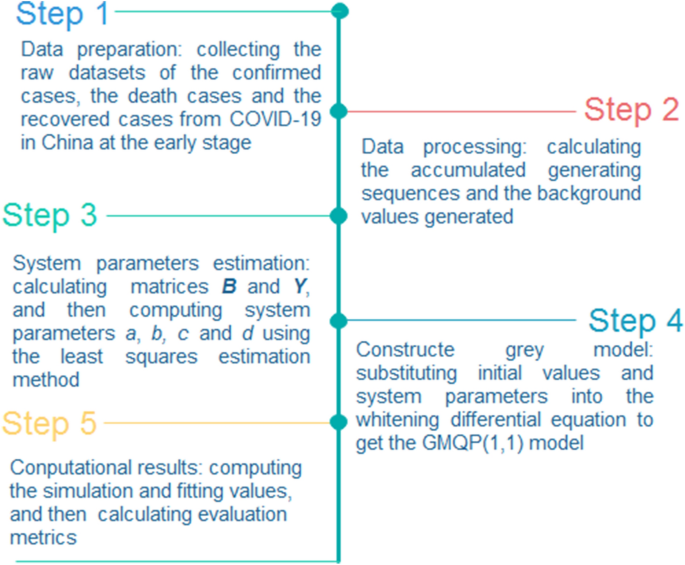

  

  The flowchart of the GMQP(1,1) model.

Validation of the GMQP(1,1) model

To validation of the feasibility of the new model, this section gives two numerical example where datasets are collected from published papers.

Example 1

In this example, data are all collected from Table 2 in Ref³⁵. where the total energy consumption in China (unit: 10000tce). These data are used to build the GM(1,1) model, the DGM(1,1) model, the NGM(1,1,k,c) model, the GVM(1,1) model and the GMQP(1,1) model. The numerical results of these grey forecasting models are displayed in the following Tables 2, 3 and 4.

Table 2 The numerical results of the energy consumption of China (unit: 10,000 tce).

Table 3 The APEs of these forecasting models in the energy consumption of China.

Table 4 The evaluation measures of these models in the energy consumption of China.

We can from Tables 2, 3, and 4 that the new model has better performance measures than other grey forecasting models in the energy consumption of China, which show that the new structure of GMQP(1,1) model can improve the precision of grey model.

Example 2

In this example, the raw data of the electricity consumption of China are collected from Table 2 in Ref.³⁶, where the twelve data are all applied to build different kinds of grey models. Similarly, the computational results and evaluation measures are listed in the following Tables 5, 6, and 7.

Table 5 The results of the electricity of China by different grey forecasting models.

Table 6 The APEs of these grey models in the electricity consumption in China.

Table 7 The evaluation measures of these models in the electricity consumption of China.

It is shown that the GM(1,1) model, the DGM(1,1) model, the NGM(1,1,k,c) model and the GMQP(1,1) model successfully catch the trend of the electricity consumption of China. Moreover, the new model has the best performance measures, while the GVM(1,1) model has the worst performance measures.

It follows from example 1 and example 2 that the new grey model has best performance measures, which shows the new grey models with a more flexible structure can be a good way of improving the accuracy of model.

Applications in the COVID-19 of China

In this section, we will use different grey forecasting models and the polynomial regression to study the confirmed cases, the death cases and the recovered cases from COVID-19 in China, which are the classical continuous grey model GM(1,1), the discrete grey model DGM(1,1), the non-homogeneous grey model NGM(1,1,k,c), the nonlinear grey Verhulst model GVM(1,1), the polynomial regression (PR) and the grey model with quadratic polynomial term GMQP(1,1). Moreover, the structure of the applications in the COVID-19 of China is shown in Fig. 2.

Figure 2

The structure of the application in the COVID-19 of China.

The confirmed cases from COVID-19 of China

In this subsection, we apply forecasting models to study the confirmed cases from COVID-19 of China. The raw data, starting 2020-01-21 to 2020-02-06, are collected from the website: http://www.nhc.gov.cn, and displayed in the following Table 8 and Fig. 3.

Figure 3

The plots of the confirmed cases from COVID-19 of China.

Table 8 The number of the confirmed cases from COVID-19 of China.

With these raw data, we can deduce the mathematical expressions of different grey model. Here we take the GMQP(1,1) model as an example to details show the modelling procedures.

Step 1 pre-process the raw data.

It follows from Table 8 that the original sequence is X⁽⁰⁾ = (291, 440, 571, 830, 1287, 1975, 2744, 4515, 5974, 7711, 9692, 11,791, 14,380, 17,205, 20,438, 24,324, 28,018). The first 14 data are used to develop the GMQP(1,1) model of the confirmed cases of COVID-19, and the remaining three data are used to test. From the definition 1, the first-order accumulating generated sequence is X⁽¹⁾ = (291, 731, 1302, 2132, 3419, 5394, 8138, 12,653, 18,627, 26,338, 36,030, 47,821, 62,201, 79,406, 99,844, 124,168, 52,186).

Step 2 System parameter estimation.

From theorem 2, and the values of X⁽⁰⁾ and X⁽¹⁾, we calculate the matrix B and the matrix Y which are given by

$$B = \left( {\begin{array}{*{20}c} { - 511} & {2.3} & {1.5} & 1 \\ { - 1016.5} & {6.3} & {2.5} & 1 \\ { - 1717} & {12.3} & {3.5} & 1 \\ { - 2775.5} & {20.3} & {4.5} & 1 \\ { - 4406.5} & {30.3} & {5.5} & 1 \\ { - 6766} & {42.3} & {6.5} & 1 \\ { - 10395.5} & {56.3} & {7.5} & 1 \\ { - 15640} & {72.3} & {8.5} & 1 \\ { - 22482.5} & {90.3} & {9.5} & 1 \\ { - 31184} & {110.3} & {10.5} & 1 \\ { - 41925.5} & {132.3} & {11.5} & 1 \\ { - 55011} & {156.3} & {12.5} & 1 \\ { - 70803.5} & {182.3} & {13.5} & 1 \\ \end{array} } \right),\quad Y = \left( {\begin{array}{*{20}c} {440} \\ {571} \\ {830} \\ {1287} \\ {1975} \\ {2744} \\ {4515} \\ {5974} \\ {7711} \\ {9692} \\ {11791} \\ {14380} \\ {17205} \\ \end{array} } \right).$$

With the help of the Eq. (17), we can obtain the values of system parameters as

$$\left\{ {\begin{array}{*{20}c} {a = 0.0116,} \\ {b = 132.7801,} \\ {c = - 536.6728,} \\ {d = 1008.4680.} \\ \end{array} } \right.$$

Step 3 Model construction.

Substituting the system parameters a, b, c and d into Eq. (12), we obtain that.

$\frac{{dx^{\left( 1 \right)} \left( t \right)}}{dt} + 0.0116x^{\left( 1 \right)} \left( t \right) = 132.7801t^{2} - 536.6728t + 1008.4680$.

And then we can obtain the expressions of Eq. (20) and Eq. (21), respectively. Therefore, we can compute the simulation and prediction values of the confirmed cases of COVID-19 of China. By a similar argument to the other grey forecasting models which are provided below.

The GM(1,1) model.

We can obtain system parameters a = -0.2441, b = 1116.9454 of the GM(1,1) model by the least squares method. And then the mathematical expression is given by.

$\frac{{dx^{\left( 1 \right)} \left( t \right)}}{dt} - 0.2441x^{\left( 1 \right)} \left( t \right) = 1116.9454$.

The DGM(1,1) model.

We directly deduce system parameters a = 0.2441, b = 1116.9454 of the DGM(1,1) model. And the mathematical formula is given by.

$x^{\left( 1 \right)} \left( k \right) = 0.2441^{k - 1} x^{\left( 0 \right)} \left( 1 \right) + \frac{{1 - 0.2441^{k - 1} }}{0.7559} \times 1116.9454$.

The NGM(1,1,k,c) model.

We can derive system parameters a = -0.1719, b = 463.7776 and c = -1124.6229 of the NGM(1,1,k,c) model. The whitening equation is built, there is.

$\frac{{dx^{\left( 1 \right)} \left( t \right)}}{dt} - 0.1719x^{\left( 1 \right)} \left( t \right) = 463.7776t - 1124.6229$.

The GVM(1,1) model.

We deduce system parameters a = -0.3820 and b = -2.0528E-6 of the GVM(1,1) model with the least squares estimation method. Further, the whitening equation is put forward, there is.

$\frac{{dx^{\left( 1 \right)} \left( t \right)}}{dt} - 0.3820x^{\left( 1 \right)} \left( t \right) = - 0.000002\left( {x^{\left( 1 \right)} \left( t \right)} \right)^{2}$.

The polynomial regression model.

We compute the values of parameters of the polynomial regression model where a = 120.9911, b = − 535.4727 and c = 916.0495, respectively. And then the mathematical expression is.

$x^{\left( 0 \right)} \left( t \right) = 120.9911t^{2} - 535.4727t + 916.0495$.

Once the specific grey forecasting models are established, the computational results and error metrics can be easily obtained which are displayed in the following Tables 9, 10, 11 and Fig. 4. The MAE_sim, MAE_fit, and MAE_all of the GMQP(1,1) model are 93.9043%, 871.5592% and 239.7146%, the MSE_sim, MSE_fit, and MSE_all of the GMQP(1,1) model are 14,610.4784%, 924,128.4138% and 185,145.0913%, the MAPE_sim, MAPE_fit, and MAPE_all of the GMQP(1,1) model are 4.8534%, 3.4346%, 4.5873%, the RMSE_sim, RMSE_fit, and RMSE_all of the GMQP(1,1) model are 7.1669%, 3.6842%, 6.6542%, the IA_sim, IA_fit, and IA_all of the GMQP(1,1) model are 0.9999%, 0.9990% and 0.9994%, the R_sim, R_fit, and R_all of the GMQP(1,1) model are 0.9998%, 0.9994% and 0.9996%, respectively.

Figure 4

The plots of the confirmed cases of COVID-19 of China.

Table 9 The computational results of the confirmed cases of COVID-19 of China.

Table 10 The APEs of different model in the confirmed cases of COVID-19 of China, (%).

Table 11 The evaluation measures of different forecasting models in the confirmed cases.

It follows from these results that the GM(1,1) model and the DGM(1,1) model has worst performance measures, the NGM(1,1,k,c) model and the GVM(1,1) model have worse performance measures, and the new model GMQP(1,1) have good performance measures. This also demonstrates that the grey model with quadratic polynomial term is more powerful to deal with the data of the confirmed cases of COVID-19 of China.

The death cases from COVID-19 of China

This subsection discusses the death cases from COVID-19 of China by employing grey models. The raw data are collected from the website: http://www.nhc.gov.cn, and displayed in the following Tables 12, 13, 14 and Fig. 5. The first 14 observations are used to build models, and the left three observation is used to test. Similar argument is applied to derive system parameters of each model, and then the mathematical expressions are given below.

Figure 5

The plots of the death cases of COVID-19 of China.

Table 12 The computational results of the death cases of COVID-19 of China.

Table 13 The Errors of different model in the death cases of COVID-19 of China, (%).

Table 14 The evaluation measures of different forecasting models in the death cases.

The GM(1,1) model.

$$\frac{{dx^{\left( 1 \right)} \left( t \right)}}{dt} - 0.2074x^{\left( 1 \right)} \left( t \right) = 37.1439$$

The DGM(1,1) model.

$$x^{\left( 1 \right)} \left( k \right) = 0.2074^{k - 1} x^{\left( 0 \right)} \left( 1 \right) + \frac{{1 - 0.2074^{k - 1} }}{0.7926} \times 37.1439$$

The NGM(1,1,k,c) model.

$$\frac{{dx^{\left( 1 \right)} \left( t \right)}}{dt} - 0.1387x^{\left( 1 \right)} \left( t \right) = 12.0569t - 15.8702$$

The GVM(1,1) model.

$$\frac{{dx^{\left( 1 \right)} \left( t \right)}}{dt} - 0.3367x^{\left( 1 \right)} \left( t \right) = - 0.000065\left( {x^{\left( 1 \right)} \left( t \right)} \right)^{2}$$

The polynomial regression model.

$$x^{\left( 0 \right)} \left( t \right) = 2.298811t^{2} - 3.0309t + 13.0714$$

The GMQP(1,1) model.

$$\frac{{dx^{\left( 1 \right)} \left( t \right)}}{dt} - 0.0369x^{\left( 1 \right)} \left( t \right) = 9.2777t^{2} + 1.7801t + 1.7402$$

When the specific mathematical expression of each model is derived, the computational results and error metrics are straightforward obtained, which are provided in the following Tables 12, 13, 14 and Fig. 5. The MAE_sim, MAE_fit, and MAE_all of the GMQP(1,1) model are 1.5865%, 3.5972% and 1.9635%, the MSE_sim, MSE_fit, and MSE_all of the GMQP(1,1) model are 3.2758%, 23.8122% and 7.1264%, the MAPE_sim, MAPE_fit, and MAPE_all of the GMQP(1,1) model are 1.6496%, 0.5921%, 1.4513%, the RMSE_sim, RMSE_fit, and RMSE_all of the GMQP(1,1) model are 2.0616%, 0.7745%, 1.8883%, the IA_sim, IA_fit, and IA_all of the GMQP(1,1) model are 1.0000%, 0.9999% and 1.0000%, the R_sim, R_fit, and R_all of the GMQP(1,1) model are 0.9999%, 0.9997% and 0.9999%, respectively.

Similarly, the GM(1,1) model, the DGM(1,1) model and the GVM(1,1) model have the worst computational results, the NGM(1,1,k,c) model has the worse computational results, and the GMQP(1,1) has the most computational results. It indicates that the new model has higher precision than the other forecasting models in the death cases from COVID-19 of China.

The recovered cases from COVID-19 in China

This subsection discusses the recovered cases from COVID-19 of China by employing grey models. The raw data are collected from the website: http://www.nhc.gov.cn, and displayed in the following Tables 15, 16, 17 and Fig. 6. The first 14 observations are used to build models, and the left three observation is used to test. Similar argument is applied to derive system parameters of each model, and then the mathematical expressions are given below.

Figure 6

The plots of the recovered cases of COVID-19 of China.

Table 15 The computational results of the recovered cases of COVID-19 of China.

Table 16 The Errors of different model in the recovered cases of COVID-19 of China, (%).

Table 17 The evaluation measures of different forecasting models in the recovered cases.

The GM(1,1) model.

$$\frac{{dx^{\left( 1 \right)} \left( t \right)}}{dt} - 0.3091x^{\left( 1 \right)} \left( t \right) = 11.9339$$

The DGM(1,1) model.

$$x^{\left( 1 \right)} \left( k \right) = 0.3091^{k - 1} x^{\left( 0 \right)} \left( 1 \right) + \frac{{1 - 0.3091^{k - 1} }}{0.6909} \times 11.9339$$

The NGM(1,1,k,c) model.

$$\frac{{dx^{\left( 1 \right)} \left( t \right)}}{dt} - 0.3067x^{\left( 1 \right)} \left( t \right) = 0.7831t + 8.1075$$

The GVM(1,1) model.

$$\frac{{dx^{\left( 1 \right)} \left( t \right)}}{dt} - 0.3359x^{\left( 1 \right)} \left( t \right) = - 0.000007\left( {x^{\left( 1 \right)} \left( t \right)} \right)^{2}$$

The polynomial regression model.

$$x^{\left( 0 \right)} \left( t \right) = 10.6655t^{2} - 85.3389t + 177.7198$$

The GMQP(1,1) model.

$$\frac{{dx^{\left( 1 \right)} \left( t \right)}}{dt} - 0.2501x^{\left( 1 \right)} \left( t \right) = 54.5571t^{2} - 19.9387t + 2.3094$$

When the specific mathematical expression of each model is derived, the computational results and error metrics are straightforward obtained, which are provided in the following Tables 15, 16, 17 and Fig. 6, respectively. The MAE_sim, MAE_fit, and MAE_all of the GMQP(1,1) model are 7.6964%, 17.8839% and 9.6065%, the MSE_sim, MSE_fit, and MSE_all of the GMQP(1,1) model are 150.7354%, 474.7209% and 211.4826%, the MAPE_sim, MAPE_fit, and MAPE_all of the GMQP(1,1) model are 4.6767%, 0.9435%, 3.9767%, the RMSE_sim, RMSE_fit, and RMSE_all of the GMQP(1,1) model are 7.1431%, 1.1304%, 6.4573%, the IA_sim, IA_fit, and IA_all of the GMQP(1,1) model are 0.9998%, 0.9999% and 0.9999%, the R_sim, R_fit, and R_all of the GMQP(1,1) model are 0.9996%, 0.9996% and 0.9999%, respectively.

Similarly, the GVM(1,1) model has the worst computational results, the GM(1,1) model, the DGM(1,1) model and the NGM(1,1,k,c) model have the better computational results, and the GMQP(1,1) has the most best computational results. It indicates that the new model has higher precision than the other forecasting models in the recovered cases from COVID-19 of China.

Conclusion

This paper studied the grey forecasting model with quadratic polynomial term, and applied it to the confirmed cases, the death cases and the recovered cases from COVID-19 of China at the early stage. By using the grey technique and some mathematical derivations, the grey basic form, the time response function and the restored values are all systematically analyzed. With raw datasets of COVID-19 in China, we compute the simulation and fitting values by different forecasting models. It follows from the computational results, we can observed the new model has higher precision than other models. This also implied that our generalized model has applicable value in the COVID-19.

In this work, the GMQP(1,1) model is an univariate grey forecasting model and some factors such as social isolation and lockdown, vaccines, active treatment cannot be considered. In addition, the integer order accumulating generated operation is used to preprocess the raw data. It is generally known that the fractional order accumulating generated operation or the new information priority to preprocess raw data can get more accurate results. Thus in the future, we will continuous consider such a model with other accumulating generated operator including new information priority, fractional accumulating generated operator. Further, other multivariate grey forecasting models can be constructed to study the COVID-19.

References

WHO, WHO to Accelerate Research and Innovation for New Coronavirus, WHO, Geneva, Switzerland, 2020, https://www.who.int/news-room/detail/06-02-2020-who-to-accelerate-research-andinnovation-for-new-coronavirus.
Castillo, O. & Melin, P. Forecasting of COVID-19 time series for countries in the world based on a hybrid approach combining the fractal dimension and fuzzy logic. Chaos Solitons Fractals 140, 110242 (2020).
Chimmula, V. & Zhang, L. Time series forecasting of COVID-19 transmission in Canada using LSTM networks. Chaos Solitons Fractals 135, 109864 (2020).
Anastassopoulou, C., Russo, L., Tsakris, A. & Siettos, C. Data-based analysis, modelling and forecasting of the COVID-19 outbreak. PLoS ONE 15(3), 1–21 (2020).
Petropoulos, F. & Makridakis, S. Forecasting the novel coronavirus COVID-19. PLoS ONE 15(3), 1–8 (2020).
Shastri, S., Singh, K., Kumar, S., Kour, P. & Mansotra, V. Time series forecasting of Covid-19 suing deep learning models: India-USA comparative case study. Chaos Solitons Fractals 140, 110227 (2020).
Wang, P., Zheng, X., Ai, G., Liu, D. & Zhu, B. Time series prediction for the epidemic trends of COVID-19 using the improved LSTM deep learning method: case studies in Russia Peru and Iran. Chaos Solitons Fractals 140, 110214 (2020).
Hawas, M. Generated time-series prediction data of COVID-19’s daily infections in Brazil by using recurrent Neural networks. Data Brief 32, 106175 (2020).
Yonar, H., Yonar, A., Tekindal, M. A. & Tekindal, M. Modeling and forecasting for the number of cases of the COVID-19 pandemic with the curve estimation models, the Box-Jenkins and exponential smoothing methods. Euras J Med Oncol 4(2), 160–165 (2019).
Melin, P., Monica, J. C., Sanchez, D. & Castillo, O. Multiple ensemble neural network models with fuzzy response aggregation for prediction COVID-19 time series: the case of Mexico. Healthcare 8, 181–193 (2020).
Sun, T. Z. & Wang, Y. Modeling COVID-19 epidemic in Heilongjiang province. China. Chaos Solitons Fractals 138, 109949 (2020).
Castillo, O. & Melin, P. A novel method for a COVID-19 classification of countries based on an intelligent fuzzy fractal approach. Healthcare 9, 196–211 (2021).
Luo, X. L., Duan, H. M. & Xu, K. A novel grey model based on traditional Richards model and its application in COVID-19. Chaos Solitons Fractals 142, 110480 (2021).
Sahin, U. & Sahin, T. Forecasting the cumulative number of confirmed cases of COVID-19 in Italy, UK and USA using fractional nonlinear grey Bernoulli model. Chaos Solitons Fractals 138, 109948 (2020).
Zhao, Y. F., Shou, M. H. & Wang, Z. X. Prediction of the number of patients infected with COVID-19 based on rolling grey Verhulst models. Int. J. Environ. Res. Public Health 17, 4582–4601 (2020).
Boccaletti, S., Ditto, W., Mindlin, G. & Atangana, A. Modeling and forecasting of epidemic spreading: the case of Covid-19 and beyond. Chaos Solitons Fractals 135, 109794 (2020).
Das, R. C. Forecasting incidences of COVID-19 using Box-Jenkins nethod for the period July 12-Septembert 11 2020: A study on highly affected countries. Chaos Solitons Fractals 140, 110248 (2020).
Nabi, K. N. Forecasting COVID-19 pandemic: a data-driven analysis. Chaos Solitons Fractals 139, 110046 (2020).
Ren, H. Y. et al. Early forecasting of the potential risk zones of COVID-19 in China’s megacities. Sci. Total Environ. 729, 138995 (2020).
Kirbas, I., Sozen, A., Tuncer, A. D. & Kazancioglu, F. S. Comparative analysis and forecasting of COVID-19 case in various European countries with ARIMA, NARNN and LSTM approaches. Chaos Solitons Fractals 138, 110015 (2020).
Pathan, R. K., Biswas, M. & Khandaker, M. U. Time series prediction of COVID-19 by mutation rate analysis using recurrent neural network-based LSTM model. Chaos Solitons Fractals 138, 110018 (2020).
Bartolomeo, N., Trerotoli, P. & Serio, G. Short-term forecast in the early stage of the COVID-19 outbreak in Italy Application of a weighted and cumulative average daily growth rate to an exponential decay model. Infect. Dis. Modell. 6, 212–221 (2021).
Alberti, T. & Faranda, D. On the uncertainty of real-time predictions of epidemic growths: A COVID-19 case study for China and Italy. Commun. Nonlinear Sci. Numer. Simulat. 90, 105372 (2020).
Deng, J. L. Control problems of grey systems. Syst. Control Lett. 1(5), 288–294 (1982).
Cui, J., Liu, S. F., Zeng, B. & Xie, N. M. A novel grey forecasting model and its optimization. Appl. Math. Model. 37, 4399–4406 (2013).
Xie, N. M., Liu, S. F., Yang, Y. J. & Quan, C. Q. On novel grey forecasting model based on non-homogeneous index sequence. Appl. Math. Model. 37, 5059–5068 (2013).
Chen, P. Y. & Yu, H. M. Foundation settlement prediction based on a novel NGM model. Math. Probl. Eng. 2014, 1–9 (2014).
Xie, N. M. & Liu, S. F. Discrete grey forecasting model and its optimization. Appl. Math. Model 33, 1173–1186 (2009).
Xie, N. M. & Liu, S. F. Discrete GM(1,1) and mechanism of grey forecasting model. Syst. Eng. Theory Practice 1(25), 93–99 (2005).
Wu, W. Q., Ma, X., Zeng, B., Wang, Y. & Cai, W. Application of the novel fractional grey model FAGMO(1,1, k) to predict China’s nuclear energy consumption. Energy 165, 223–234 (2018).
Hu, N. Y. & Ye, Y. C. Improved unequal-interval grey Verhulst model and its application. J. Grey Syst. 1(30), 175–185 (2018).
Zou, G. Y. & Wei, Y. Integrated time-varying grey Verhulst model and its application. J. Grey Syst. 1, 9–16 (2019).
Wang, Z. X. & Li, Q. Modelling the nonlinear relationship between CO2 emissions and economic growth using a PSO algorithm-based grey Verhulst model. J. Clean. Prod. 207, 214–224 (2019).
Deng JL, Fundations of grey theory, Huazhong University of Science and Technology Press, 2002, In Chinese.
Guo, X. J., Liu, S. F., Wu, L. F. & Tang, L. L. A grey NGM(1,1, k) self-memory coupling prediction model for energy consumption prediction. Sci. World J. 301032, 1–12 (2014).
Zeng, B., Meng, W. & Tong, M. Y. A self-adaptive intelligence grey predictive model with alterable structure and its application. Eng. Appl. Artif. Intell. 50, 236–244 (2016).
Funding
This work did not receive any specific funding, and also was not performed as part of the employment of the authors.
Author information
Authors and Affiliations
Contributions
Conceptualization, J.B. Zhang; methodology, Z.Y. Jiang; matlab code, J.B. Zhang; data curation, Z.Y. Jiang; Writing, J.B. Zhang. All authors read and approved the final manuscript.
Corresponding author
Ethics declarations
Competing interests
The authors declare no competing interests.
Additional information
Publisher's note
Springer Nature remains neutral with regard to jurisdictional claims in published maps and institutional affiliations.
Rights and permissions
Open Access This article is licensed under a Creative Commons Attribution 4.0 International License, which permits use, sharing, adaptation, distribution and reproduction in any medium or format, as long as you give appropriate credit to the original author(s) and the source, provide a link to the Creative Commons licence, and indicate if changes were made. The images or other third party material in this article are included in the article's Creative Commons licence, unless indicated otherwise in a credit line to the material. If material is not included in the article's Creative Commons licence and your intended use is not permitted by statutory regulation or exceeds the permitted use, you will need to obtain permission directly from the copyright holder. To view a copy of this licence, visit http://creativecommons.org/licenses/by/4.0/.
About this article
Cite this article
Zhang, J., Jiang, Z. A new grey quadratic polynomial model and its application in the COVID-19 in China. Sci Rep 11, 12588 (2021). https://doi.org/10.1038/s41598-021-91970-1
Received:
Accepted:
Published:
Version of record:
DOI: https://doi.org/10.1038/s41598-021-91970-1
This article is cited by
-
An adaptive non-equidistant grey model with four parameters and its applications in deformation monitoring
Scientific Reports (2025)
Evaluating the impact of COVID-19 outbreak on hepatitis B and forecasting the epidemiological trend in mainland China: a causal analysis
BMC Public Health (2024)
Deathdaily: A Python Package Index for predicting the number of daily COVID-19 deaths
Network Modeling Analysis in Health Informatics and Bioinformatics (2022)