Integrating numerical models with deep learning techniques for flood risk assessment

Abstract

Floods are among the natural disasters that pose significant threats to both urban and rural infrastructure, as well as the lives and properties of individuals. Streamflow prediction is essential for obtaining hydrological information and is critical for a variety of water resource projects. While precise daily streamflow predictions are indispensable, forecasting streamflow according to the limited data can help reduce computational time and enhance the efficacy of flood early warning systems. The purpose of this research is streamflow forecasting with the Long Short-Term Memory (LSTM) approach for the next 20 years. The peak streamflow extracted from the LSTM model was entered into HEC-RAS software and obtained flood zone maps and hazard maps. Furthermore, the effectiveness of the proposed method was assessed through statistical analysis, including the coefficient of determination (R²), Mean absolute error (MAE), Root mean square error (RMSE), Nash–Sutcliffe efficiency (NSE), Kling-Gupta efficiency (KGE) and Mean bias error (MBE). In addition to the numerical comparison, the models were evaluated. Their performances were evaluated based on graphical plotting, including scatter plot, violin plot, box plot and Taylor diagram. In the chosen model (MD-8), the values RMSE (m³/s), R², MAE, NSE, KGE and MBE are 4.57, 0.98, 2.56, 0.98, 0.94 and 0.17 during the training period, respectively, and 6.40, 0.92, 3.81, 0.89, 0.87 and 0.09 during the testing period, respectively. The simulation was tailored to the daily streamflow series of the Nesa river in Iran, which spans over 40 years. It is evaluated the results of generating flood zone maps using both the 2D HEC-RAS and LSTM models. The water inflow volume into the reservoir was found to be 76.3 million cubic meters, based on the peak streamflow predicted by the LSTM approach. The present model results demonstrate that the volume of water inflow into the reservoir for return periods of 25, 100 and 500 years were calculated as 76.26, 148.73 and 149.22 million cubic meters, respectively. Additionally, the Difference Flood Hazard (DFH) maps are obtained, illustrating the difference in flood hazard under various conditions.

Introduction

Enhancing flood forecasting with the integration of process-based and Deep Learning Models is a critical focus in studying natural disasters. Floods pose various destructive consequences that put everything associated with humans at risk¹. Many deaths and significant harm to livelihoods, property, infrastructure, and utility services result from this danger². The occurrence of floods is typically attributed to natural events, resulting from severe weather conditions that lead to the overflowing of main rivers and their smaller branches, inundating adjacent areas³.

The flood phenomenon is also considered one of these natural disasters, which has increased in number and extent over the years due to human intervention. In general, the phenomenon of flood occurs when the soil, and plants cannot absorb rain or runoff from melting snow and the rivers do not have the capacity to pass these waters. The overflow of these waters from the main bed of the river and the occupation of the plains around it can damage residential houses, offices and facilities, ultimately putting human lives at risk. Although arid and semi-arid regions make up the majority of Iran, it has always been exposed to flood risks. Due to flood modeling and forecasting, it is necessary to identify the factors causing and intensifying it, investigate the damages, and prevent and reduce the damages⁴. Flood modeling involves a technical approach that can offer accurate details about the flood profile, encompassing factors that influence flooding, such as rainfall, surface waterflow, and characteristics of the watershed⁵.

The Hydrologic Engineering Center’s River Analysis System (HEC-RAS) software is considered as one of the most widely used tools for investigating flood simulations because of its significantly improved capacity to simulate canals and natural rivers^6,7.

Flood modelling necessitates a two-dimensional modeling; in this aspect, HEC-RAS represents groundbreaking research in the subcontinent and throughout the world. The water surface elevation determines the accuracy of the flood map. Although GIS and HEC-RAS 1D models may be inadequate to portray actual circumstances, automated floodplain mapping and analysis using HEC-RAS (2D) will provide more efficient, effective, and consistent results⁸.

In a research by Sarchani et al. in 2020, they combined flood study with one-dimensional and two-dimensional HEC-RAS on a river in Greece named Crete to calculate the flood risk map in the catchment area. To ensure the accuracy of parameters such as the Manning coefficient of the river, they used a simultaneous analysis method. The results of the simulation can be helpful in creating flood risk maps⁹. While this study focuses on natural flood dynamics, dam failure scenarios (e.g., structural breaches or overtopping) could exacerbate inundation risks downstream. For instance, in 2022, Hosseinzadeh-Tabrizi et al. utilized a 2D HEC-RAS model to simulate the flood downstream of the Sattar Khan Dam, located in the northwest of Iran. The importance of this issue is the location of Ahar city downstream of the dam. Their research investigated the population and infrastructure of this area based on two dam failure scenarios. The results indicated that certain population centers downstream of the dam area are at flooding risk in case of dam break. The study calculated the arrival time of the flood and the maximum velocity in the affected regions. The aim of their research was to aid in the development of a comprehensive crisis management plan¹⁰. In 2022, Mohammadi et al. assessed the performance of numerical simulations in replicating river flood zones within the Azarshahr Qushqura River area. They also contrasted the 1D and 2D hydraulic models of HEC-RAS. The flood flow hydraulic characteristics, such as the velocity and depth of the flow at various cross sections, were assessed. Findings indicated that the two-dimensional model HEC-RAS displayed the least error in the water surface level (flow depth) in comparison with other hydraulic parameters of flood flow, as opposed to the one-dimensional model¹¹.

In a study by Vashist and Singh in 2023, a 2D hydrodynamic model was utilized for charting flood inundation for the Krishna River. Flood maps were generated using Digital Elevation Models (DEMs) with different resolutions. The impact of alterations in upstream boundary data on the extent of the flooded area was also investigated in their study. The simulated outcomes obtained from the 12.5-m resolution DEM demonstrated reasonable agreement with the validation data and closely matched the documented inundated regions².

The Keser watershed was the focus of a 2023 research study, which involved numerical modeling of flood hydrographs. This was conducted to aid in disaster risk reduction and the efficient management of water resources, particularly for the development of an Emergency Action Plan (EAP) for the Tugu Dam. This study focused on calculating peak discharge. Based on the calculations, the flood discharge calculated utilizing the HEC-HMS model was 451.1 m³/s. The values of peak discharge calculated using the Gamma, Nakayasu and Snyder methods were 410.4, 424.2 and 439.4 m³/s, respectively¹².

In 2023, Shaikh et al. evaluated the flood event of 2006 in the low-lying areas of Surat city, India, using the HEC-RAS model for 2D hydrodynamic modeling within a GIS framework. In this study, a 30-meter resolution digital elevation model of Surat city was obtained from SRTM data. The discharge hydrograph from the Ukai Dam during the flood event, along with normal depth, was considered as the upstream and downstream boundary conditions for the simulation. The simulated flood results, when compared to the observed flood mapping of 2006, showed correlation coefficient values of R² = 0.96, NSE = 0.90, and RMSE = 0.66 m¹³.

In 2024, El-Bagoury and Gad assessed the risks of flash floods, calculating the volume of flood discharge in two drainage basins in southeastern Egypt that had experienced several devastating floods. Their study revealed that the effects of floods caused by torrential rains were more severe in areas near the mouth of the Nile River. To mitigate these risks, they recommended the construction of five dams, each with a height of ten meters, to create a water storage lake¹⁴.

In the last decade, information-based frameworks such as Machine Learning (ML) and Deep Learning (DL) approaches have attracted attention in the fields of hydrological studies and water management¹⁵. Numerous factors aided the development of DL in hydrology, which include: (a) availability of substantial amounts of information, (b) quick development in the concurrent processing systems with multi-core capabilities, GPU technology, (c) specific software frameworks including TensorFlow and keras that allow developing tiered deep learning structures without investigating complicated mathematical aspects, (d) effective optimization results attaining nearly optimal outcomes, and (e) enhanced regularization techniques to counteract overfitting¹⁶.

The development of the LSTM model involved utilizing deep learning techniques, and it has been operationalized as a conventional machine learning method to forecast daily inflow. After that, it became very popular as one of the successful deep learners in the field of artificial neural networks. The term “deep learning” was first introduced to Descartes Machine Learning and Artificial Neural Networks by Eisenberg and her colleagues¹⁷. It should be noted that various discussions have been carried out regarding the use of machine learning (ML) models across different areas of hydrology and flow estimation¹⁸. Neural network approaches, such as LSTM, due to their consecutive structure, can exploit complex properties more efficiently than traditional machine learning models, assuming that adequate information is supplied¹⁹. Moreover, Liu et al.²⁰ announced that the Long Short-Term Memory model, which features built-in storage, is capable of learning and retaining long-term connections in the input-output relationship across various climate conditions. Cheng et al.²¹ used ML algorithms to forecast long-term flow on both a daily and monthly basis. Neural network models, recurrent neural networks, and a robust technique for understanding time dynamics for an extended duration or capturing nonlinear correlations are used to predict flow in terms of daily and monthly rates associated with a prolonged duration. Findings of this study showed that the LSTM managed to advance daily flow predicting and would be useful in supporting a framework for decision processes for hydrological management.

A recent study was conducted in the region of southwestern India called Kerala, which has an annual mean rainfall of approximately 3,000 mm, using deep neural networks. In this research, flood forecasting has been investigated using in-depth training. Forecasting was analyzed using meteorological data focusing on LSTM and RNN-GRU approaches and evaluated by RMSE and MAE criteria²².

The long short-term memory (LSTM) network has been widely utilized due to its recurrent architecture and distinctive gating system. This approach has demonstrated significant potential in hydrological forecasting, including flood alerts and river level predictions²³. Latif and Ahmed utilized deep learning and machine learning algorithms to predict the daily inflow of the Dukan Dam on the Zab River in the Kurdistan Region of Iraq. They compared the performance of the deep learning algorithm with that of the enhanced Boosted Regression Tree (BRT). The results indicated that the root mean square error (RMSE) for the Long Short-Term Memory (LSTM) model demonstrated significantly superior accuracy. The LSTM model exhibited high reliability and accuracy, making it a valuable tool for predictions²⁴. Li et al.²⁵ proposed anew hybrid method that merges traditional physical models with historical data to train LSTM networks. Using the NAM hydrological model and the HD hydraulic model, on the Jinhua basin in China to evaluate the effectiveness of LSTM models trained on different datasets. Results show that LSTM models trained on mixed datasets, particularly those with a simulated-to-measured data ratio of less than 2:1, perform better, achieving lower RMSE and MAE values. This hybrid model represents a significant advancement in flood forecasting, offering a viable solution to issues of computational efficiency and data scarcity. Dtissibe et al.¹⁶ has experienced on the Far-North region of Cameroon, flood prediction techniques in the area are mainly based on physical models and often produce inadequate outcomes. This study investigates the use of artificial intelligence, particularly machine learning and deep learning algorithms, to enhance flood forecasting. The research compares different models, such as one-dimensional convolutional neural networks, Long Short-Term Memory (LSTM), and Multi-Layer Perceptron, utilizing temperature and rainfall time series data as inputs. Performance is assessed using metrics like Nash–Sutcliffe Efficiency and Root Mean Squared Error. The results show that the LSTM model excels in both short-term and long-term flood forecasting, exhibiting strong performance and generalization capabilities.

Although the utilization of deep learning and LSTM model concepts has grown in popularity, an extensive discussion of deep learning concepts, methodologies, deployments, challenges, research deficiencies, and future possibilities and its combination with numerical models in hydrology is still lacking, which is the main reason for this review.

Consequently, this study’s contribution is centered on employing the LSTM model to determine the daily peak streamflow and generate flood hazard maps through 2D HEC-RAS. Subsequently, the hazard maps depict potential flooding cases with return periods of 25, 100, and 500 years. By examining the flood hazard maps and the reservoir volume, it is tried to evaluate the capability of the reservoir to contain the flood volume.

Materials and methods

Introduction of study area

Streamflow prediction of the Nesa river which is located in the country of Iran between longitudes 55°17 to 61°11’E and latitudes 27°52° to 34°7°N with an area of 760 square kilometers is considered a pertinent case study to fulfill the aims of this investigation (Fig. 1). Additionally, the average altitude of the basin is about 2424.7 m. The length of the main river under study is about 22.4 km and the tributary is 12.4 km.

The average annual rainfall in the area is 400 mm, and in most places it is less than 100 mm, with the highest amount is in the winter season. The maximum monthly rainfall is in January, February and March and the minimum is in July and August. The economic development of the Bam region greatly depends on the Nesa Dam and the flow downstream, which also has significant environmental and hydrological implications.

Fig. 1

Representation of the study area geographical location using ArcGIS 10.8 software.

For the purpose of simulating streamflow forecasting, a range of daily discharge data spanning from 1978 to 2019 was gathered for this research. The total number of daily discharge data points is 14,976. Out of this total, 11,980 are selected as training data and 2996 are designated as test data.

Fig. 2

The Yalkhari station discharge values on a daily basis for 40 years.

The Yalkhari hydrometric station is located 8 km from the Nesa Dam. Figure 2 shows the daily discharge during these years at this specific station. The years 1979 and 2002 lacked data and were therefore excluded from the calculations. The hydrological characteristics of the research area are presented in Table 1.

Table 1 Hydrological characteristics of the Nesa river basin.

Methodology

In hydrology, the process of streamflow prediction is extremely important^26,27. In this study, an investigation is conducted to assess how different forecasting models perform. The LSTM network is frequently utilized for handling time-series data due to its impressive memory capacity, giving it inherent benefits for processing such data²⁸. Nowadays, significant progress has been achieved in methodologies and practical applications through the advancements of deep learning. According to the results obtained, it is obvious that the implementation of the created LSTM model demonstrates significant and improved accuracy, making it a dependable and trustworthy tool for forecasting streamflow and other hydrological factors. As mentioned earlier in the literature review, numerous research studies confirm the significance and reliability of LSTM, either on its own or when integrated with other algorithms in hybrid models²⁴. LSTM has proven to be an effective tool for sequence modeling in various tasks, as it has the ability to retain past information for prediction purposes. In their study, Fu et al.²⁹ introduced the outcomes of an improved LSTM model and demonstrated its clear benefits in handling continuous streamflow data during the arid periods in the Kelantan River, located in Malaysia. Rainfall and inflow were the input parameters of their study.

The implementation of the model can be effective, depending on prior studies. the authors compared²⁴ BRT and DL prediction models using daily discharge data from Dokan Dam, on the Lesser Zab River. Training and testing subsets were created from thedataset. The data was divided into two parts: 80% for training and 20% for testing. The authors¹⁶ utilized a dataset comprising historical temperature and rainfall time series from the Far-North region of Cameroon. Temperature and rainfall values were recorded weekly or monthly from 1980 to 2020. The dataset was divided as follows: 80% was used for model training and 20% for model testing. In the present study, the ratio of 80:20 was considered for the dataset.

With repeated tests, the ratio of 80:20 was found to yield the best results for the dataset. Other ratios, such as 70:30, decreased the accuracy and negatively impacted the model’s performance.

In this part, there is a description of the Long Short-Term Memory Network (LSTM) used for forecasting streamflow and modeling 2D HEC-RAS, a widely used hydraulic model for flood zone mapping and inundation. The purpose of this research is to utilize a deep learning model for long-term forecasting and to integrate it with the HEC-RAS numerical model. This approach aims to assess potential measures for mitigating high-risk floods while considering the presence of a reservoir. By using deep learning and a large dataset, the LSTM (Long Short-Term Memory) model was identified as suitable for sequential data analysis, particularly in tasks such as time series prediction, due to its superior performance in these contexts.

Deep learning, as a subset of machine learning, is particularly effective for solving complex problems. Previous studies and analyses of time series data indicate that the LSTM model is the most effective solution for the specific needs of this research. It is important to note that deep neural networks, including LSTM, require substantial amounts of data and powerful hardware to process this data effectively in order to achieve optimal performance. Consequently, the LSTM model was selected as the primary model after thorough investigation.

In the present study, the LSTM model was developed using Python and Keras. The model consists of four levels of neurons (200-100-80-30) and activation functions. The model underwent training for 100 epochs, after which it made predictions using the testing data. Nine different models (MD) have been proposed to choose the most accurate input parameter (Table 2).

Table 2 Representation of daily inflow time series data considered for proposed model combinations.

Introduction of LSTM model

Long Short-Term Memory (LSTM), suggested by Hochreiter and Schmidhuber³⁰, is a modified version designed to address the limitations of the Recurrent Neural Network (RNN) and overcome the issues of gradient explosion or vanishing³¹. The LSTM model developed in the present study includes three layers: input, hidden, and output layers. The LSTM model’s design is shown in Fig. 3^32,33. The sequential input x = {x₁, x₂, …, x_N} and the output chain y = {y₁, y₂…, y_N} are linked by the forget door, which determines whether the current data should beforgotten or remembered. At a particular time stage t, the calculation can be performed in the following manner³⁴:

Fig. 3

Representation of the LSTM layer.

$$\:{\text{h}}_{\text{t}}=\text{H}\left({\text{w}}_{\text{h}\text{h}}{\text{h}}_{\text{t}-1}+{\text{w}}_{\text{h}\text{x}}{\text{x}}_{\text{t}}+\:{\text{b}}_{\text{h}}\:\right)\:\:\:\:\:\:\:\:\:\:\:\:\:\:\text{t}>0$$

(1)

Where b_h is the forget door bias, W_hh and W_hx represent the forget weight matrix and the forget-hidden weight matrix, and H represents the nonlinear activation function. Tanh and ReLU are the most common choices for H activation in recursive networks. The parameter $\:{\:\stackrel{\sim}{\text{c}}}_{\text{t}}$memorizes the up-to-date data and the forget door f_t concludes the data updating. They are presented as follows:

$$\:{\text{f}}_{\text{t}}={\upsigma\:}\left({\text{w}}_{\text{x}\text{f}}{\text{x}}_{\text{t}}+\:{\text{w}}_{\text{h}\text{f}}{\text{h}}_{\text{t}-1}+\:{\text{b}}_{\text{f}}\right)$$

(2)

$$\:{\:\stackrel{\sim}{\text{c}}}_{\text{t}}=\text{t}\text{a}\text{n}\text{h}\left({\text{w}}_{\text{x}\text{i}}{\text{x}}_{\text{t}}+\:{\text{w}}_{\text{h}\text{i}}{\text{h}}_{\text{t}-1}+\:{\text{b}}_{\text{i}}\right)$$

(3)

where W_xf and W_hf denote the weight matrix. The weights and biases are also displayed with the W and b symbol. The bias vectors for the input door and the cell state update are depicted sequentially as b_f and b_i. Afterward, the new state of the memory cell, c_t, is updated in the following manner:

$$\:{\:\text{c}}_{\text{t}}=\left({\text{f}}_{\text{t}}\text{*}{\text{c}}_{\text{t}-1}+\:{\text{i}}_{\text{t}\:}*{\:\stackrel{\sim}{\text{c}}}_{\text{t}}\right)$$

(4)

where c_t−1 represents the previous state of the memory cell, and the * represents element-wise product. The output door handles the output activations at the end. The hidden layer, which is sent to a subsequent time stage, is defined as follows:

$$\:{\text{h}}_{\text{t}}={\text{o}}_{\text{t}}\text{*}\text{t}\text{a}\text{n}\text{h}\left({\text{c}}_{\text{t}}\right)$$

(5)

$$\:{\text{o}}_{\text{t}}={\upsigma\:}\left({\text{w}}_{\text{x}0}{\text{x}}_{\text{t}}+\:{\text{w}}_{\text{h}0}{\text{h}}_{\text{t}-1}+\:{\text{b}}_{0}\right)$$

(6)

where the output weight matrix is represented as w_xo, b_o is the output door bias and w_ho represents the output-concealed weight matrix.

Implementation of LSTM model

The procedure for the implementation of the LSTM model consists of the following steps;

• i. To begin, the sequence data containing input parameters needs to be loaded, with the time steps aligned with the day value associated with streamflow. In LSTM, the model learns to remember relevant information from past time steps (or previous elements in the sequence) and uses that information to make predictions or generate output at the current time step. Each time step represents a moment in time or a specific position in the sequence and is typically represented as a column in the input data matrix.

• ii. Next, it’s time to split the training and testing data into separate partitions. In the present study, the proposed LSTM model has been trained on 80% of the time-series data, and 20% of the time-series data has been chosen to test the mFig.  Fig. 4.

  Fig. 4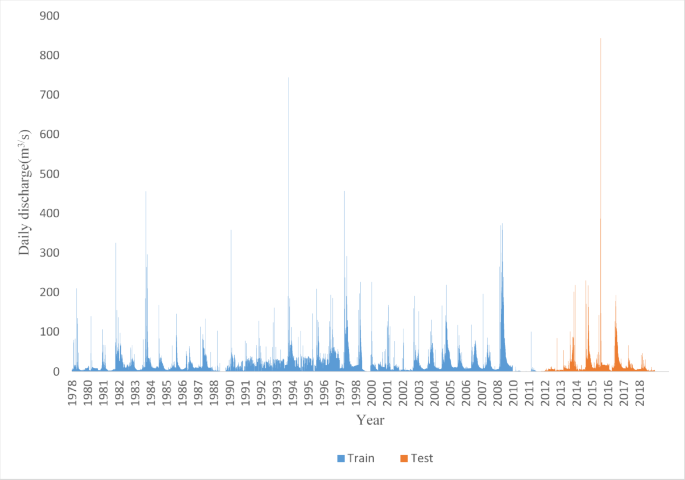

  

  The Yalkhari station discharge values on a daily basis for 40 years.

• iii. The next step involves normalizing the data in order to achieve a zero mean and unit variance, which will improve the fitting and prevent the training from diverging.

• iv. Finally, the responses and predictors need to be prepared.

  $$\:{\text{Q}}_{\text{t}}=\text{f}\left({\text{Q}}_{\text{t}-1\:}.{\text{Q}}_{\text{t}-2\:}.\dots\:.{\text{Q}}_{\text{t}-\text{m}\:}\right)$$

  (7)

After repeated stages, different hyper-parameters are set. The hyper-parameters used in the LSTM model are presented in Table 3 as follows:

Table 3 The presentation of Hyper-parameters used in the LSTM.

Model performance evaluation

Performance evaluation criteria in hydrological studies can be classified into various categories, each with corresponding mathematical relationships. To assess the performance and accuracy of the model, a range of statistical and hydrological criteria were utilized to derive quantitative results. These include: the Mean Absolute Error (MAE), coefficient of determination (R²), Root Mean Square Error (RMSE), the Nash Sutcliffe model Efficiency coefficient (NSE), Kling-Gupta efficiency (KGE) and Mean bias error (MBE), which were employed to evaluate the performance and accuracy of the model. In an ideal model, the MAE should be minimized and close to zero, while the R² should be maximized and close to one. This indicates that the model accounts for a considerable amount of the variance in the data. These criteria are calculated using the following Eqs^35,36.

$$\:\text{M}\text{A}\text{E}=\frac{\:1}{\text{N}}\sum\:\left|{\text{x}}_{\text{i}}-{\text{y}}_{\text{i}}\right|\:\:\:\:\:\:\:\:\:$$

(8)

$$\begin{aligned}\text{R}^{2}=\frac{\sum^{\text{N}}_{\text{i}=1}(\text{X}_{\text{i}}-\overline{\text{X}})(\text{y}_{\text{i}}-\overline{\text{y}})}{\sqrt{\sum^{\text{N}}_{\text{i}=1}(\text{X}_{\text{i}}-\overline{\text{X}})^{2}\sum^{\text{N}}_{\text{i}=1}(\text{y}_{\text{i}}-\overline{\text{y}})^{2}}} \end{aligned}$$

(9)

$$\:\text{R}\text{M}\text{S}\text{E}\:=\:\sqrt{\:\:\frac{1}{\text{N}}{\sum\:}_{\text{i}=1}^{\text{N}}{\left(\text{x}\text{i}-\text{y}\text{i}\right)}^{2}}$$

(10)

$$\:\text{N}\text{S}\text{E}=1-\:\frac{{\sum\:}_{\text{i}=1}^{\text{N}}{\left({\text{y}}_{\text{i}}-{\text{x}}_{\text{i}}\right)}^{2}}{{\sum\:}_{\text{i}=1}^{\text{N}}{\left({\text{x}}_{\text{i}}-\stackrel{-}{\text{x}}\right)}^{2}}$$

(11)

$$\:\text{K}\text{G}\text{E}=1-\:\sqrt{(\text{R}{\left({\text{x}}_{\text{i}}{.\text{y}}_{\text{i}})-1\right)}^{2}+{\left(\frac{var{\left({\text{y}}_{\text{i}}\right)}^{\frac{1}{2}}}{var{\left({\text{x}}_{\text{i}}\right)}^{\frac{1}{2}}}-1\right)}^{2}+{\left(\frac{\stackrel{-}{\text{y}}}{\stackrel{-}{\text{x}}}-1\right)}^{2}\:}$$

(12)

$$\:\text{M}\text{B}\text{E}=\frac{\:1}{\text{N}}\sum\:(\:{\text{x}}_{\text{i}}-{\text{y}}_{\text{i}})$$

(13)

In which x_i and y_i represent the observational and computational values in the chronological step of i, respectively. N denotes the total number steps, while x and y represent the average computational and observational values, respectively, in the given order.

Numerical model: 2D HEC-RAS

The peak discharges for the basin, in addition to the land use maps, were utilized as inputs for the 2D HEC-RAS approach, which allowed the simulation of the variability and distribution of the flow pathway. The model then generated flood velocity and depth maps to determine the regions that were flooded and determine locations with hazards¹⁴. The two-dimensional HEC-RAS model has been employed for the analysis of reservoir operations³⁷, and to enhance the urban flood risk assessment maps³⁸. The 2D mesh’s flow field is computed using the diffusion wave approximation approach, which results in a shorter computation time and a reduction in the possibility of model instability in comparison to the shallow water Eqs^14,39. The computational domain is divided into grid cells, and HEC-RAS produces a comprehensive hydraulic property table for all cells. The model’s water surface profiles, created with various hydraulic design elements, can assist decision-makers in investing resources to better prepare for disasters and enhance the life quality. This is achieved by analyzing the severity of flooding and flood inundation areas to improve the level of preparedness. In this research, the diffusion wave equations were used in 2D HEC-RAS v 6.5 Beta, ArcGIS v 10.8 was utilized to create flood depth maps.

In the application of the HEC-RAS model, geometric data and flow data are two fundamental components. Creating geometric data, which determines the river channel, longitudinal profile of the river, left and right banks of the floodplain, and drawing the cross-section and flow direction, is the first step in simulating the flood for different return periods using the HEC-RAS model. Topographic maps and DEM are utilized to transfer the output to the HEC-RAS software. Subsequently, the RAS mapper tool is utilized to obtain the extent of flood protection and hazard maps. The necessity of flood study in the period of different returns is to measure or estimate the magnitude of peak flows. By analyzing flood frequency based on instantaneous maximum values and probability distribution functions, the estimated best instantaneous maximum discharge can be determined. The river bed boundary is determined using topographic maps, GIS, and HEC-RAS 2D. Floodplain maps offer valuable information about the flood’s characteristics and its impact on the floodplain, allowing for timely warnings to be issued during periods of flood risk.

Simulations

The two-dimensional unsteady HEC-RAS model was established by integrating the Digital Elevation Model (DEM) of the research area into the RAS Mapper to generate the topographicalrepresentation. For the 30-meter resolution DEM, 31,428 cells were produced for cell sizes dx and dy equal to 30 m and Manning’s roughness coefficient (n) as 0.033. Each mesh should have only one computation point.

The model has been updated with a new geometry file for the terrain layer geometry data. The model development also requires 2D surface roughness, Boundary Conditions (BCs), and unsteady flow data as other parameters. The input for surface roughness includes the Manning’s roughness coefficient. To generate the mesh and map inundation, a 2D flow area is specified for the terrain by outlining a polygon around the study area involving all the relevant reaches. The flow area parameters were used to generate a computational mesh in the 2D flow area. Figure 5 displays the two-dimensional flow area that was generated using a 30-meter DEM. During flood simulation, the hydraulic model is calibrated by varying Manning’s coefficient for flood zones and channels. Upon completing mesh generation, boundary conditions are applied to the 2D flow area for performing unsteady flow analysis. Three boundary conditions, one downstream and two upstream, have been applied close to the 2D flow region as displayed in Fig. 5. All necessary details are provided by flow data that is considered for the unsteady analysis of the flow. For the boundary condition, a time series of discharge in the form of a hydrograph (an input hydrograph) has been considered in the simulation.

Fig. 5

2D area plan and boundary conditions of the Nesa River using HEC-RAS v 6.5 Beta software.

Based on discharge data from the Yalkhari Hydrometric Station, the best fitting distribution was determined according to three criteria: Anderson-Darling, Kolmogorov-Smirnov, and Kai-Squire for return periods of 2, 25, 100, 500, and 1000 estimates. After completing the data inputs, The HEC-RAS model was employed for the purpose of conducting an extensive analysis of the flow. The model generated a comprehensive report of the analysis, which included information on the flow depth, discharge values at each cross section, and other simulation details. The examination of the region inundated under various return-period flood events is based on the peak flows derived from frequency analysis executed through the utilization of Easyfit and HEC-HMS v 4.10 software. The maximum instantaneous discharges at the Nesa river for different periods were obtained using the Gamma distribution, as presented in Table 4.

Table 4 Gamma distribution results of maximum discharge values (M³ /s).

To run the 2D HEC-RAS model, programs including the unsteady flow simulation, geometry preprocessor, floodplain mapping, postprocessor, and simulation period should be determined for the evaluation of unsteady flow. Computational settings include the hydrograph output interval, computation interval, and mesh generation for a 30 m resolution DEM terrain layer and a 2D area flow with mesh provided for the simulations. The calculation interval is an important parameter in unsteady flow calculations. It should be selected in a way that ensures accuracy and stability according to the Courant condition, and produces satisfactory results⁴⁰. In order to specify the optimal computation interval and maintain stability and accuracy, the computation interval was set to 5 min. While this study utilized ground-based hydrological data, future work could incorporate remote sensing datasets (e.g., satellite-derived rainfall from GPM or topographic data from LiDAR) to enhance spatial resolution and real-time flood monitoring. Such integration could refine DEM accuracy and provide dynamic inputs for LSTM models. As a result, applying remote sensing datasets could increase the accuracy of LSTM prediction results.

Results

Utilization of LSTM model for forecasting analysis

the empirical evidence indicates that the proposed Long Short-Term Memory (LSTM) model not only exhibits significant superiority in the analysis of consistent streamflow data during the arid season but also demonstrates commendable proficiency in discerning data characteristics within the highly variable streamflow data encountered in the wet season. The advanced deep learning LSTM model results demonstrated that, in most cases, it could accurately forecast extreme events. In the present study, the Nesa River dataset has been used to develop and apply the LSTM model for daily streamflow forecasting. The daily streamflow over the past 40 years is the chosen input parameter, and the daily streamflow prediction output parameter is extracted for the next 20 years.

The analysis was conducted across nine models, focusing on the average value, standard deviation, and skewness of the data. The standard deviation serves as a measure of dispersion or variability within the dataset. The results suggest that nearly all the models exhibit similar levels of dispersion. Furthermore, the positive skewness value indicates that the data is inclined towards larger values as presented in Table 5.

Table 5 Statistical analysis in the introduced models.

According to Table 6, MD-2 and MD-8 were selected for analytical and graphical comparison because the statistical indicators in MD-2 demonstrated better results than those of the other models. Additionally, MD-2 demonstrated better results than the first seven models, so it was compared with the best LSTM model which is MD-8.

Considering all the models have been previously utilized and MD-8 outperformed the others, a forecast is made for the next 20 years, which corresponds to about 8000 time steps (with a lag of four, consisting of 2000 time steps each). It is presented as model MD-9. According to the LSTM results, MD-8, regarding the training dataset, the R² = 0.98, RMSE = 4.57, NSE = 0.98, KGE = 0.94, MBE = 0.17 and MAE = 2.56, respectively. For the testing dataset, R² = 0.92, RMSE = 6.40, NSE = 0.89, KGE = 0.87, MBE = 0.09 and MAE = 3.81 respectively. Table 6 shows the performance of the training and testing sets for forecasting daily streamflow using the LSTM method.

Table 6 The performance evaluation for forecasting daily streamflow using LSTM.

According to Table 6, the output results of the model show that the R² values remain relatively constant from the first model (MD-1) to the seventh model (MD-7). Among these models, MD-2 has the lowest mean absolute error (MAE) and is therefore the basis for comparison with model MD-8, which has the best performance.

Additional to the statistical parameters stated in Eqs. (8–13), the correctness of the investigated models (MD-2 and MD-8) and other models were validated using the scatter plot, violin plot and box plot and Taylor diagrams.

The techniques’ scatter plots demonstrate that for training and testing data MD-2 and MD-8, Figs. 6 and 7, followed by LSTM, can forecast streamflow more accurately than alternative models due to the values generated being closer to the optimal line. In the remaining models, scatter plots were drawn according to Fig. 8.

Fig. 6

Streamflow forecasting scatter plots through training with LSTM (a) MD-2, (b) MD-8.

Fig. 7

Streamflow forecasting scatter plots through testing with LSTM (a) MD-2, (b) MD-8.

Fig. 8

Streamflow forecasting scatter plots through training with LSTM (a). MD-1, (b). MD-3, (c). MD-4, (d). MD-5, (e). MD-6, (f). MD-7, (g). MD-9 and testing with LSTM (a1). MD-1, (b1). MD-3, (c1). MD-4, (d1). MD-5, (e1). MD-6, (f1). MD-7, (g1). MD-9.

The LSTM model was trained and tested on MD-1 to MD-9 time series data. The violin plot and box plot distribution of the observed and predicted streamflow during the training and testing periods for all models, Fig. 9. Correlation coefficients and standard deviation values between predicted and observed values might be shown in this diagram to aid in the detecting of changes between the two values. In Violin and Box plots, the MD-8 model captured the extreme values better during the training and testing than the MD-2 and other models. In the middle of the chart, there is a box that shows the median, quartiles, and maximum and minimum data. The violin chart allows us to observe the distribution of data along the vertical axis to estimate the actual density of data and to identify the points where data is most concentrated. The violin shape shows the density of data distribution. The MD-2 distribution, in comparison to both prediction and observation, shows that the test distributions are slightly wider than the training distribution, indicating more variability in the test, and the MD-8 distribution for prediction and observation data is relatively similar.

Fig. 9

Streamflow forecasting Violin Diagram and Box plots through training and testing with LSTM (a). Violin Diagram Train MD-1 to MD-9, (b). Violin Diagram Test MD-1 to MD-9, (c). Box plot TrainMD-1 to MD-9, (d). Box plot Test MD-1 to MD-9.

All models represented the data distribution well. The predicted data in the MD-8 model is more similar to the observed data, which indicates that the MD-8 model performs better during training and testing than the MD-2 model, Fig. 9. In addition, the efficiency of the model was compared using the Taylor diagram, Fig. 10. The Taylor diagram provides a comparative assessment of the model’s performance on different datasets and for different configurations. The concluded MD-8 model showed the highest accuracy. The Taylor diagram illustrates normalized standard deviation (radial axes), correlation coefficients (angular axes), and root mean square error (RMSE) (dashed arcs). A closer proximity to the reference point (observed data) indicates higher model accuracy. In the Taylor diagram, the distance from the center represents the ratio of the standard deviation of the predicted data compared to that of the observed data. The larger the radial distance, the more the predicted data aligns with the observed data, highlighting the differences between the predicted and observed values.

Fig. 10

Streamflow forecasting Taylor Diagram through training and testing with LSTM (a) MD-2, (b) MD-8.

The Taylor diagram with the observed and predicted streamflow during the training and testing periods for MD-1 to MD-9 is depicted in Fig. 11.

Fig. 11

Streamflow forecasting Taylor Diagram through training and testing with LSTM (a). Train MD-1 to MD-9, (b). Test MD-1 to MD-9.

The Beeswarm plot with the observed and predicted streamflow during the training and testing periods for all models is presented in Fig. 12. In Beeswarm plots, the observed and predicted data for both training and testing datasets are analyzed. The numerical distribution diagram illustrates the flow distribution of the numerical variable. This chart allows for a direct visual comparison of the distributions of the numerical variable between the two categories.

Fig. 12

Streamflow forecasting Beeswarm plot through training and testing with LSTM. (a) Train MD-1 to MD-2, (b) Test MD-1 to MD-9.

While the Beeswarm plot shows the distribution, incorporating summary statistics like the mean or median for each group would make the comparison more concrete. In the MD-8 plot, the training data (Train-MD-8) distribution is centered lower on the scale and shows a wider spread (more variability). In contrast, the testing data (Test-MD-8) distribution is centered higher on the scale with a narrower spread (less variability). There are slight differences in the distributions compared to the MD-9 chart, which could be attributed to changes in the model architecture, hyperparameters, or the data used.

The Train-MD-2 data shows a higher concentration of points in the lower flow range, with a greater density of blue points towards the bottom of the distribution. While most points are concentrated at the lower end, there is still a noticeable spread extending towards higher flow values, indicating a range of flow magnitudes within the training set. In contrast, the Test-MD-2 data exhibits a wider spread across the flow range compared to Train-MD-2. Red points are observed from very low flow values all the way to much higher values. The density of points in Test-MD-2 is less pronounced at the lower flow range compared to Train-MD-2. Although there are still points at the lower end, they are more dispersed. Regarding higher flow values, Test-MD-2 clearly shows a greater presence of higher flow values than Train-MD-2. In conclusion, the bee swarm diagram reveals notable differences in flow distribution between Train-MD-2 and Test-MD-2. The wider spread and presence of higher flow values in the test set suggest potential challenges for model generalization and underscore the importance of understanding the underlying data characteristics.

The distribution of the training data (MD-9) appears to be centered lower on the scale and shows a wider spread or variability. In contrast, the testing data (MD-9) distribution is centered higher on the scale compared to the training data (MD-9). It also seems to have a narrower spread, suggesting less variability in the values. This observation indicates that the model might be generalizing well to unseen data. Additionally, in the test dataset for MD-9, the model shows a lower error, which indicates better performance. The differences in spread could suggest that the training dataset (MD-9) is more sensitive to variations in the data.

The time series plots displayed in Fig. 13 indicate that the LSTM model accurately captures the discharge observations’ pattern. Figure 14 shows streamflow forecasting for the next 20 years with LSTM.

Fig. 13

(a) The comparison of the training set and (b) the comparison of the testing set of MD-8 for LSTM Observed against Predicted daily streamflow.

Fig. 14

Streamflow forecasting for the next 20 years by LSTM.

Finally, the peak discharge predicted by LSTM training was entered into the HEC-RAS software. The flood zone and inundation maps were created by modeling the peak discharge. The results indicate that the volume entering the reservoir is 76.73 million cubic meters, as illustrated in Fig. 15.

Fig. 15

Flood zone and Inundation map with Streamflow forecasting for the Nesa River by LSTM using HEC-RAS v 6.5 Beta software.

Forecasting analysis utilizing 2D HEC-RAS

The purpose of conducting hydraulic studies is to investigate and identify the flood zone of the Nesa River through hydraulic modeling. To achieve this goal, the HEC-RAS software has the capability to simulate one-dimensional, two-dimensional and mixed flow. Version 6.5 Beta of the HEC-RAS hydraulic model has built-in features that can be used to easily perform the flood zone process. DEM resolutions of 30 m were utilized in simulations to create the inundation map for the 1998 flood (due to the devastating and historical floods in this river, theflood of 1998 was considered as the reference flood) and the floods with different return periods. Two boundary conditions were specified upstream, and one boundary condition was specified downstream. The boundary conditions were considered upstream of the flow hydrograph and downstream of the stage hydrograph. The level of the reservoir bed plus the flood depth were used in these boundary conditions. Maps of flood area size, depth, and flow rate are displayed according to the digital elevation model (DEM) with a resolution of 30 m. The maps involve floods with a return period of 25 to 500 years. Finally, for the flood event in 1998 with a 25-year return period, the volume entering the reservoir is equal to 26.62 and 76.26 million cubic meters, respectively. The surface area under the flood is 9.11 and 13.59 square kilometers, as shown in Fig. 16. The reservoir area measures 3,902,280 square meters.

Fig. 16

Flood zone and Inundation map for (a) the flood event in 1998 and (b) 25-year return period of Nesa River using HEC-RAS v 6.5 Beta software.

The volume entering the reservoir with a return period of 100 and 500 years is equal to 148.73 and 149.22 million cubic meters, respectively. The surface area under the flood is 19.76 and 20.96 square kilometers, respectively. The time of arrival of the flood to the reservoir is about 22 h in the return period of 100 years (Fig. 17).

Fig. 17

Flood zone and Inundation map with (a) 100, and (b) 500 years return and (c) arrival time flood to reservoir in 100 years return period of Nesa River using HEC-RAS v 6.5 Beta software.

The results of the volume, area, and arrival time of the reservoir during different periods are listed in Table 7. Based on the flood area in various return periods and the flood of 1998, it can be concluded that the percentage of flood area with a return period of 100 years will increase significantly (approximately 216.9%) compared to the flood of 1998 in this region. Also, the volume of the reservoir in the return period of 100 years will reach 148.73 million cubic meters, which according to the average volume of the reservoir (103.44 million cubic meters), will reach about 252.17 million cubic meters, which will be about 84.17 million cubic meters in excess of the capacity of the reservoir, and it is necessary to think of measures in the overflow of the dam.

Table 7 Results of 2D HEC-RAS model.

Mapping of flood hazard

The first step in flood hazard assessment is to recognize regions that are prone to flooding. From a reliable point of view, determine the areas flooding is a hydraulic hydrological modeling that can be applied to determine the flood area, depth and velocity of water. Flood hazard indicates the intensity of flood that will cause damage and casualties. There are several methods for flood hazard zoning^41,42. In this research, the Australian method was used, which is a combination of two main flow parameters (depth and velocity) considered as criteria for flood hazard assessment. Based on that, six hazard levels are presented according to Table 8; Fig. 18⁴³, .

Table 8 Levels of flood risk⁴³.

Fig. 18

Illustration of general curves for flood hazard vulnerability⁴³.

According to the guidelines, flood hazard maps were generated for the flood of 1998 and for the 100 and 500-year return periods. Additionally, the predicted flood was determined using LSTM. These maps were created by taking into account two parameters: depth and velocity. Flood hazard maps were created in two cases, flow hydrograph and fixed profile (peak discharge). In both cases, the Nesa River was classified as one of the most hazardous rivers and assigned to group H6, indicating that all types of buildings were considered vulnerable to failure. Thus, the possibility of dam failure is a significant concern. Figures 19, 20, 21 and 22 represent flood hazard maps produced for the geographical region of the Nesa River.

Fig. 19

Representation of flood hazard maps produced for the geographical region of the Nesa River the flood of 1998, (a) D*V ) m*m/s) event plan, (b) flood hazard event plan, (c) peak discharge hazard event plan using HEC-RAS v 6.5 Beta software.

Fig. 20

Representation of flood hazard maps produced for the geographical region of the Nesa River with a return period of 100 years. (a) D*V ) m*m/s) event plan, (b) flood hazard event plan, (c) peak discharge hazard event plan using HEC-RAS v 6.5 Beta software.

Fig. 21

Representation of flood hazard maps produced for the geographical region of the Nesa River with a return period of 500 years. (a) D*V ) m*m/s) event plan, (b) flood hazard event plan, (c) peak discharge hazard event plan using HEC-RAS v 6.5 Beta software.

Fig. 22

Representation of flood hazard maps produced for the geographical region of the Nesa River with discharge predicted by LSTM. (a) D*V ) m*m/s) event plan, (b) flood hazard event plan, (c) peak discharge hazard event plan using HEC-RAS v 6.5 Beta software.

Finally, by transferring these maps to QGIS v 3.22.5 software, Difference Flood Hazard (DFH) maps have been obtained. DFH refers to the difference between the amount of damage caused by a flood and the amount of damage that can occur in reality. The DFH for the return period of 100 years, the streamflow predicted by LSTM, and the flood of 1998 are shown in Fig. 23.

DFH maps illustrate the difference in flood hazard under various conditions. DFH was added to the DEM maps in raster form. Figure 23 (a) shows a smaller difference compared to Fig. 23 (b).

Fig. 23

(a) DFH map for flood with return period of 100 years and the flood event in 1998), (b) DFH map for flood with return period of 100 years and inflow predicted in LSTM of the Nesa River using ArcGIS 10.8 software.

In Fig. 23, the Difference Flood Hazard (DFH) map illustrates that the most affected regions are the river banks, the parts of the main channel, and the spiral parts of the river. The DFH in the 100-year return period and the streamflow predicted by LSTM in Fig. 23 (b) show that the flood hazard would reach its highest level at the junction of two river branches. In other words, it can be said that due to the high-risk potential of floods in the return period of 100 and 500 years, and considering that the region is mountainous and downstream is also connected to the reservoir, it is necessary to pay special attention to the proper management of water resources and flood warning systems.

Discussion

As previously discussed, the primary research question of this paper is how to predict the streamflow based on the time series dataset using Long Short-Term Memory (LSTM) networks, as well as the assessment of flood zones and inundation resulting from HEC-RAS 2D. Nine different models were developed using daily streamflow data with Long Short-Term Memory (LSTM) networks, which generated predictions for the next 20 years. Additional to the statistical parameters, the correctness of the investigated models (MD-2 and MD-8) and another models were validated using the scatter plot, violin plot and box plot and Taylor diagrams. Comparisons and analyses were conducted between the MD-2 and the best-performing model (MD-8). Finally, MD-9 was chosen as the research target. Its model can be extended for practical applications.

A comparison of LSTM between MD-2 and MD-8 with LSTM streamflow forecasts was provided in the analysis. The results show that the deep learning models demonstrate good streamflow prediction ability. This attribute makes deep learning have great potential in hydrological prediction and analysis. The MD-8 model proposed in this paper has fairly high prediction accuracy and also provides a reliable prediction interval.

Based on the literature review, in 2020, Zhu et al. carried out a study, and the findings demonstrated that the hybrid LSTM integrated with the Gaussian process would improve forecasting precision and offer a flexible prediction interval, which is extremely important for planning and administration in water resources. This conclusion is similar to the results of the present study⁴⁴. In another investigation in 2023²⁴, , the LSTM model was created and utilized on the Dokan dam dataset for predicting daily reservoir inflow. The chosen input variable was the daily reservoir inflow. According to the LSTM results, regarding the training dataset, RMSE = 34.1, R² = 0.98, and NSE = 0.98, respectively. For the testing dataset, RMSE = 19.1, R² = 0.99, and NSE = 0.98, respectively. This illustrates the performance of the testing set for predicting daily reservoir inflow using the developed LSTM method. It is to be mentioned that in the present study, the statistical analysis gave more reasonably results. While the current study focuses on historical streamflow data, climate change could significantly alter rainfall patterns and flood frequencies in the Nesa River basin. For instance, increased precipitation intensity, as projected in arid regions like Iran may amplify flood risks. Future iterations of this model could integrate climate projections to assess long-term reservoir capacity and floodplain management under changing climatic conditions.

Box plot and violin plot are both powerful tools for data analysis. In Fig. 9, the box plot displays the distribution and dispersion of data by showing the median, quartiles, and potential outliers, based on the maximum and minimum values. The standard deviation of the models MD-2 and MD-8 related to testing data varies between 22.16 and 20.87, with a correlation between 0.86 and 0.92, and for training data varies between 27.94 and 32.26, with a correlation between 0.85 and 0.98. Theseplots in Fig. 9 (b, h) show that MD-8 is able to predict daily flow better than MD-2, with predictions closer to observations and a correlation of 0.92 for the test data and a correlation of 0.98 for the training data.

As well as, a Taylor diagram and a violin plot provide a deeper understanding of the data distribution by combining a box plot with a density plot, allowing for a visualization of the data’s distribution shape along with its summary statistics. The MD-8 model captured the values better during the training than the other models. The performance of the MD-9 model was similar to that of the MD-8. The statistical indicators in MD-8 confirm that it is suitable for flow prediction.

The qualitative performance evaluation of the models was achieved by visual observations such as Taylor diagram, scatter plot, violin plot and box plot, and quantitative evaluations were carried out using different statistical and hydrological performance indices, namely, root mean square error (RMSE), coefficient of determination (R²), the Nash–Sutcliffe coefficient of efficiency (NSE), the Mean Absolute Error (MAE), Kling-Gupta efficiency (KGE), Mean bias error (MBE) were employed to evaluate the performance and accuracy of the model. After obtaining the predicted daily streamflow from the LSTM model, the volume of water inflow into the reservoir was 76.3 million cubic meters, and for return periods of 25, 100, and 500 years, calculations were made. In the following, the difference flood hazard (DFH) revealed that many parts of the river are serpentine, necessitating further study in this locality.

Conclusion

This research was conducted with the aim of flood forecasting and risk assessment, as well as determining the vulnerability of the Nesa River to floods. Data accumulated from the Nesa River basin over a period of 40 years has been split into two sets for training and testing purposes. The LSTM model was applied to predict streamflow for the next 20 years. The peak streamflow extracted from the LSTM model was then inputted into the 2D HEC-RAS software to generate flood zone maps and hazard maps. Regarding to evaluate the performance of the present model, two statistical criteria including MAE and R² were calculated for both the training and test datasets. The examination of the region inundated during various return-period flood events is informed by the peak discharge values derived from frequency analysis performed using Easyfit and HEC-HMS software. The maximum instantaneous discharges at Nesa river for different periods were obtained using the Gamma distribution. Flood modeling was done using 2D HEC-RAS, and the required hydraulic parameters (depth, velocity, etc.) were extracted from this model. Using these parameters and following the existing standard in this field, flood zoning and flood hazard maps were prepared. To ensure graphical congruence of the fulfillment of different methods, observed and predicted daily streamflow data were applied to create scatter plots and time series graphs. The results of generating flood zone maps using both the 2D HEC-RAS and LSTM approaches were evaluated. Results indicate that the volume of water inflow into the reservoir 76.3 million cubic meters by the LSTM model and for return periods of 25, 100 and 500 years were calculated as 76.26, 148.73 and 149.22 million cubic meters, respectively. The results show that the volume of water inflow into the reservoir is 76.3 million cubic meters according to the LSTM model. The calculated values for return periods of 25, 100, and 500 years are 76.26, 148.73, and 149.22 million cubic meters, respectively. The surface area under the flood is 9.11, 19.76, and 20.96 square kilometers, respectively. The arrival time of the flood to the reservoir is about 22 h for the return periods of 100 and 500 years. Examining the flood hazard maps shows that based on the ADRH method, the flood is classified as H6, which means it is unsafe for people and vehicles. All types of buildings are regarded as susceptible to failure. In the following, the Difference Flood Hazard (DFH) maps illustrate that the most affected areas are the banks of this river, the parts of the main channel, and the spiral parts of the river. According to the DFH map, the villages around the river are at risk of flooding. However, due to the mountainous terrain of the area, a significant portion of the flood volume is stored in the reservoir to prevent damage to the downstream areas.

Finally, the present study indicated that LSTM methods are capable of predicting daily streamflow in this study field. Consequently, the models are deemed appropriate for forecasting streamflow and, as a result, for the effective management of flood events. The utilization of deep learning frameworks in conjunction with hydrological models ought to be augmented to enhance the efficacy of long-term streamflow predictions. CNN (Convolutional Neural Networks) can be implemented on spatiotemporal data, such as satellite imagery of flood-prone areas, to identify patterns and predict flood occurrences. BiLSTM (Bidirectional Long Short-Term Memory) and GRU (Gated Recurrent Unit) are other deep learning models recommended for integration with hydrological assessments to improve predictive performance in flood forecasting. Although LSTM was selected for its proven efficacy in sequential data, alternative architectures like GRU or hybrid models (e.g., CNN-LSTM) could further validate our results. For example, GRUs offer computational efficiency, while CNNs excel at spatial feature extraction from raster data. Future studies may explore these models to assess robustness across diverse hydrological regimes.

Together, these technologies create a robust framework that enhances the accuracy of flood predictions, ultimately aiding in the mitigation of flood impacts. The use of numerical models, such as SWAT and HEC-HMS, in combination with various deep learning algorithms, such as BiLSTM and GRU, can provide valuable information for researchers, especially given the lack of information and limitations in this area.

It is to be mentioned that the exact effects of climate change can be considered as a suggestion for further research.

References

Cabrera, J. S. and Han Soo Lee. Flood-prone area assessment using GIS-based multi-criteria analysis: A case study in Davao Oriental, Philippines. Water 11(11), 2203.https://doi.org/10.3390/w11112203 (2019).
Vashist, K. & Singh, K. K. HEC-RAS 2D modeling for flood inundation mapping: a case study of the Krishna river basin. Water Pract. Technol. 18 (4), 831–844. https://doi.org/10.2166/wpt.2023.048 (2023).
Teng, J. et al. and S. J. E. M. Kim. Flood inundation modelling: A review of methods, recent advances and uncertainty analysis. Environmental modelling & software 90, 201–216. https://doi.org/10.1016/j.envsoft.2017.01.006 (2017).
Mokhtari Hashi, H. Zoning of flood risk in human and economic activities centers of South Khorasan Province using the fuzzy logic system. Geogr. Environ. Plann. 27 (1), 199–216. https://doi.org/10.22108/gep.2016.21366 (2016).
Al-Hussein, Asaad, A. M., Shuhab Khan, K., Ncibi, N., Hamdi & Younes Hamed. and. Flood analysis using HEC-RAS and HEC-HMS: a case study of Khazir River (Middle East—Northern Iraq). Water 14(22), 3779. https://doi.org/10.3390/w14223779 (2022).
Dasallas, L., Kim, Y. & Hyunuk An. and. Case study of HEC-RAS 1D–2D coupling simulation: 2002 Baeksan flood event in Korea. Water 11(10), 2048. https://doi.org/10.3390/w11102048 (2019).
Albu, L. M., Enea, A., Iosub, M. & Iuliana-Gabriela, B. Dam breach size comparison for flood simulations. A HEC-RAS based, GIS approach for Drăcșani Lake, Sitna River, Romania. Water 12(4), 1090. https://doi.org/10.3390/w12041090 (2020).
Chowdhury, R., Mawla, A. A., Ankon, A. B. M. I. & Hossain Flood mapping for Jamuna river in Bangladesh using Hec-Ras 1d/2d coupled model to assess the adverse effect of the flood on the agriculture and infrastructure of the Jamuna flood plain. Issue 12 Ser. I. 16, 12–24. https://doi.org/10.9790/2380-1612011224 (2023).
Sarchani, S., Seiradakis, K., Coulibaly, P. & Ioannis Tsanis. and. Flood inundation mapping in an ungauged basin. Water 12(6), 1532. https://doi.org/10.3390/w12061532 (2020).
Hosseinzadeh-Tabrizi, S. & Alireza Mahnaz Ghaeini-Hessaroeyeh, and Maryam Ziaadini-Dashtekhaki. Numerical simulation of dam-breach flood waves. Appl. Water Sci. 12 (5), 100. https://doi.org/10.1007/s13201-022-01623-5 (2022).
Mohammadi, M. A., Ebrahimnezhadian, H., Asgarkhan Maskan, M. & Vaziri, V. Evaluation of the one and two-dimensional HEC-RAS models’ performance in determining flood zone of rivers. : fa187–fa200. https://doi.org/10.47176/jwss.26.2.43941 (2022).
Ansori, M., Bagus, U., Lasminto & Anak Agung Gde Kartika. Flood hydrograph analysis using synthetic unit hydrograph, Hec-Hms, and Hec-Ras 2D unsteady flow precipitation on-Grid model for disaster risk mitigation. Geomate J. 25 (107), 50–58. https://doi.org/10.21660/2023.107.3719 (2023).
Shaikh, A., Aziz, A. I., Pathan, S. I. et al. Application of latest HEC-RAS version 6 for 2D hydrodynamic modeling through GIS framework: a case study from coastal urban floodplain in India. Model. Earth Syst. Environ. 9 (1), 1369–1385. https://doi.org/10.1007/s40808-022-01567-4 (2023).
El-Bagoury, H. & Gad, A. Integrated hydrological modeling for watershed analysis, flood prediction, and mitigation using meteorological and morphometric data, SCS-CN, HEC-HMS/RAS, and QGIS. Water 16(2) 356. https://doi.org/10.3390/w16020356 (2024).
Tripathy, K. P., Mishra, A. K. Deep learning in hydrology and water resources disciplines: concepts, methods, applications, and research directions. J. Hydrol. 628, 130458. https://doi.org/10.1016/j.jhydrol.2023.130458 (2024).
Dtissibe, F. Y. et al. A comparative study of machine learning and deep learning methods for flood forecasting in the Far-North region. Cameroon Sci. Afr. 23, e02053. https://doi.org/10.1016/j.sciaf.2023.e02053 (2024).
Schmidhuber, J. Deep learning in neural networks: An overview. Neural networks 61, 85–117. https://doi.org/10.1016/j.neunet.2014.09.003 (2015).
Fang, W. et al. Examining the applicability of different sampling techniques in the development of decomposition-based streamflow forecasting models. J. Hydrol. 568, 534–550. https://doi.org/10.1016/j.jhydrol.2018.11.020 (2019).
Rahimzad, M. et al. Performance comparison of an LSTM-based deep learning model versus conventional machine learning algorithms for streamflow forecasting. Water Resour. Manage 35 (12), 4167–4187. https://doi.org/10.1007/s11269-021-02937-w (2021).
Liu, M. et al. The applicability of LSTM-KNN model for real-time flood forecasting in different climate zones in China. Water 12(2), 440. https://doi.org/10.3390/w12020440 (2020).
Cheng, M., Fang, F., Kinouchi, T. & Navon, I. M. Pain. Long lead-time daily and monthly streamflow forecasting using machine learning methods. J. Hydrol. 590, 125376. https://doi.org/10.1016/j.jhydrol.2020.125376 (2020).
Chitra, P. and Uma Maheswari Rajasekaran. Time-series analysis and flood prediction using a deep learning approach. In 2022 International Conference on Wireless Communications Signal Processing and Networking (WiSPNET). 139–142. https://doi.org/10.1109/WiSPNET54241.2022.9767102 (IEEE, 2022).
Luppichini, M., Barsanti, M., Giannecchini, R. & Bini, M. Deep learning models to predict flood events in fast-flowing watersheds. Sci. Total Environ. 813, 151885. https://doi.org/10.1016/j.scitotenv.2021.151885 (2022).
Latif, S. & Dashti Streamflow prediction utilizing deep learning and machine learning algorithms for sustainable water supply management. Water Resour. Manage 37 (8), 3227–3241. https://doi.org/10.1007/s11269-023-03499-9 (2023).
Li, J., Wu, G., Zhang, Y. & Shi, W. Optimizing flood predictions by integrating LSTM and physical-based models with mixed historical and simulated data. Heliyon 10(13). https://doi.org/10.1016/j.heliyon.2024.e33669 (2024).
Bakhshi Ostadkalayeh, Fatemeh, S., Moradi, A., Asadi, A. M., Nia & Somayeh Taheri. Performance improvement of LSTM-based deep learning model for streamflow forecasting using Kalman filtering. Water Resour. Manage. 37, 3111–3127. https://doi.org/10.1007/s11269-023-03492-2 (2023).
Goodarzi, M., Reza, M. J., Poorattar, M., Vazirian & Talebi, A. Evaluation of a weather forecasting model and HEC-HMS for flood forecasting: case study of Talesh catchment. Appl. Water Sci. 14 (2), 34. https://doi.org/10.1007/s13201-023-02079-x (2024).
Guo, Y. et al. Research on precipitation forecast based on LSTM–CP combined model. Sustainability 13(21), 11596. https://doi.org/10.3390/su132111596 (2021).
Fu, M., Ding, T. F. Z. & Salih, S. Q. Nadhir Al-Ansari, and Zaher mundher Yaseen. Deep learning data-intelligence model based on adjusted forecasting window scale: application in daily streamflow simulation. Ieee Access. 8, 32632–32651. https://doi.org/10.1109/ACCESS.2020.2974406 (2020).
Hochreiter, S. & Schmidhuber, J. Long short-term memory neural computation. 9 (8): 1735–1780. https://doi.org/10.1162/neco.1997.9.8.1735. (1997).
Song, T. et al. Flash floodforecasting based on long short-term memory networks. Water 12 (1), 109. https://doi.org/10.3390/w12010109 (2019).
Hu, C. et al. Deep learning with a long short-term memory networks approach for rainfall-runoff simulation. Water 10(11), 1543. https://doi.org/10.3390/w10111543 (2018).
Akbari Asanjan, Ata, T., Yang, K., Hsu, S., Sorooshian, J. & Lin Short-term precipitation forecast based on the PERSIANN system and LSTM recurrent neural networks. J. Geophys. Research: Atmos. 123 (22), 12–543. https://doi.org/10.1029/2018JD028375 (2018).
Fang, Z., Wang, Y., Peng, L. & Haoyuan Hong. Predicting flood susceptibility using LSTM neural networks. J. Hydrol. 594, 125734. https://doi.org/10.1016/j.jhydrol.2020.125734 (2021).
Fadaei-Kermani, E. & Ghaeini-Hessaroeyeh, M. Fuzzy nearest neighbor approach for drought monitoring and assessment. Appl. Water Sci. 10 (6), 1–8. https://doi.org/10.1007/s13201-020-01212-4 (2020).
Situ, Z. et al. Improving urban flood prediction using LSTM-DeepLabv3 + and bayesian optimization with Spatiotemporal feature fusion. J. Hydrol. 630, 130743. https://doi.org/10.1016/j.jhydrol.2024.130743 (2024).
Garcia, M. Integrating reservoir operations and flood modeling with HEC-RAS 2D. Water 12, 8. https://doi.org/10.3390/w12082259 (2020).
Mihu-Pintilie, A., Cîmpianu, C. I. & Stoleriu, C. C. Martín Núñez Pérez, and Larisa Elena Paveluc. Using high-density LiDAR data and 2D streamflow hydraulic modeling to improve urban flood hazard maps: A HEC-RAS multi-scenario approach. Water 11(9), 1832. https://doi.org/10.3390/w11091832 (2019).
Brunner, G. W. HEC-RAS River Analysis System. (US Army Corps of Engineers, Hydrologic Engineering Center,2016).
Brunner, G. W. CEIWR-HEC HEC-RAS river analysis system: User’s manual version 6.0. US Army Corps of Engineers Institute for Water Resources, HEC, January: Davis, CA, USA. (2021).
Afsous, M., Bambaeichi, S. & Kakavand, E. Manual for Providing Flood Risk Maps, No.821. Deputy of Technical, Infrastructure and Production Affairs. (Ministry of Energy, Water and Wastewater Standards and Projects Bureau, 2020).
Zahran, S., Gooda, E. A. & AbdelMeged, N. Modeling Al-Qaraqoul Canal before and after rehabilitation using HEC-RAS. Sci. Rep. 14 (1), 14760. https://doi.org/10.1038/s41598-024-74721-w (2024).
Australian Disaster Resilience Handbook Collection (ADRHC). ‘Flood Hazard guidline 7 – 3’, p. 30, (2017).
Zhu, S., Luo, X., Yuan, X. & Xu, Z. An improved long short-term memory network for streamflow forecasting in the upper Yangtze river. Stoch. Env. Res. Risk Assess. 34, 1313–1329. https://doi.org/10.1007/s00477-020-01766-4 (2020).
Author information
Authors and Affiliations
Contributions
All authors contributed to the study conception and design. Material preparation, data collection and analysis were performed by all authors. The first draft of the manuscript was written by the first author (Fatemeh Kordi), and all authors commented on previous versions of the manuscript (Ehsan Fadaei-Kermani, Mahnaz Ghaeini-Hessaroeyeh, Hamed Farhadi). The final revisions have been applied by Ehsan Fadaei-Kermani and Mahnaz Ghaeini-Hessaroeyeh. Moreover, all authors have read and approved the final manuscript.
Corresponding author
Ethics declarations
Competing interests
The authors declare no competing interests.
Consent to participate
The authors give their consent to take part in this project.
Consent for publication
The authors declare their consent to publication of the manuscript by the journal of “Scientific Reports”.
Additional information
Publisher’s note
Springer Nature remains neutral with regard to jurisdictional claims in published maps and institutional affiliations.
Rights and permissions
Open Access This article is licensed under a Creative Commons Attribution-NonCommercial-NoDerivatives 4.0 International License, which permits any non-commercial use, sharing, distribution and reproduction in any medium or format, as long as you give appropriate credit to the original author(s) and the source, provide a link to the Creative Commons licence, and indicate if you modified the licensed material. You do not have permission under this licence to share adapted material derived from this article or parts of it. The images or other third party material in this article are included in the article’s Creative Commons licence, unless indicated otherwise in a credit line to the material. If material is not included in the article’s Creative Commons licence and your intended use is not permitted by statutory regulation or exceeds the permitted use, you will need to obtain permission directly from the copyright holder. To view a copy of this licence, visit http://creativecommons.org/licenses/by-nc-nd/4.0/.
About this article
Cite this article
Kordi-Karimabadi, F., Fadaei-Kermani, E., Ghaeini-Hessaroeyeh, M. et al. Integrating numerical models with deep learning techniques for flood risk assessment. Sci Rep 15, 8913 (2025). https://doi.org/10.1038/s41598-025-93465-9
Received:
Accepted:
Published:
Version of record:
DOI: https://doi.org/10.1038/s41598-025-93465-9