
Abstract
Identification of cohorts at higher risk of cancer can enable earlier diagnosis of the disease, which significantly improves patient outcomes. In this study, we select nine cancer sites with high incidence of late-stage diagnosis or worsening survival rates, and where there are currently no national screening programmes. We use data from medical helplines (NHS 111) and secondary care appointments from all hospitals in England. We show that features based on information captured in NHS 111 calls are among the most influential in driving predictions of a future cancer diagnosis. Our predictive models exhibit good discrimination, ranging from 0.69 (ovarian cancer) to 0.83 (oesophageal cancer). We present an approach of constructing cohorts at higher risk of cancer based on feature importance and considering possible bias in model results. This approach is flexible and can be tailored based on data availability and the group the intervention targets (i.e. symptomatic or asymptomatic patients).
Introduction
Improving specificity in identifying cohorts at higher risk of developing cancer could increase rates of early diagnosis and allow more focused interventions to be delivered. However, diagnosing people early is complicated as early-stage symptoms can be harder to definitively attribute to cancer pathology. This means a very large number of individuals would need to be tested to detect a relatively small number of cancers, rendering using such symptoms impractical as a basis for symptomatic case finding or population level screening programmes. To achieve more accurate cancer incidence prediction, the last decade has seen a proliferation of machine learning models trained with unprecedented access to large datasets and computing power. Previous research, in that vein, has typically either (i) used routinely collected data, from either secondary or primary care1,2,3,4,5,6,7,8,9,10,11, or (ii) used imaging and/or biomarker/genetic data, which are limited to small segments of the population (e.g. those with specific comorbidities)12,13,14,15,16.
Previous research has provided a wealth of findings highlighting the promise of using machine learning for cancer risk prediction. Both these approaches are not however without their limitations when it comes to early identification of cohorts at higher risk of cancer among the general population. This is because secondary care data may only capture cancer specific events that are picked up quite late in the patient pathway, which could result in worse outcomes. On the other hand, focusing only on primary care data may miss the useful information included in secondary care data, which has shown promise in recent research17. Moreover, the use of data that are available for only a small segment of the population is unsuitable for identifying high risk cohorts at the population level.
To optimise identification of high-risk cohorts, a combination of both primary and secondary care data, at the population level, would be preferable. This approach could capture both symptoms and lifestyle factors, as well as detailed comorbidities, which have previously been shown to be useful signals for predicting future cancer incidence. In the absence of access to national level primary care data, we decided to use National Health Service (NHS) data from medical helplines, specifically, NHS 111 calls data18. The NHS 111 medical helplines aim to provide an alternative channel for UK patients seeking advice on urgent (but not life-threatening) medical needs beyond what is available in Accident & Emergency (A&E) departments or the 999 emergency lines. In 23/24 alone there were 21.8 million calls to those lines in England19. In that sense, NHS 111 lines have similarities, in terms of scope and aim, with medical helplines in other countries including Australia (Healthdirect), Germany (116117), Canada (telephone triage services) or Sweden (Healthcare guide 1177).
The NHS 111 calls dataset records symptoms individuals were concerned about and could provide early insights of undiagnosed cancer, signals which we would miss if relying solely on secondary care data. Our research progresses the field in this direction by matching secondary care data—capturing important features including pre-existing comorbidities, frequency of hospital appointments and demographics - to NHS 111 calls data. This is the first time that data from medical helplines have been used to predict future cancer incidence. Data from NHS 111 calls have the additional advantage that they are not “clinician-initiated data” in the sense that “they do not reflect data created through specific actions (or inactions) or insights of the clinician”. This is significant because recent research has made a compelling case that predictions based on “clinician-initiated data” may have limited added value, compared to “what the average clinician would decide for the average similar patient”20.
Alongside the rich data from secondary care, we construct detailed patient pathways covering five years of patient history. By doing so, we capture comorbidities and frequency of interactions with the healthcare system. There is some evidence that frequency of interactions in secondary care may reflect the number of missed appointments in primary care, arguably a reflection of patient behaviour, and, as such, including frequency of secondary care interactions could help capture relevant patient behaviour towards their health21.
We focus on nine cancers (bladder, head and neck, kidney, lymphoma, myeloma, oesophageal, ovarian, pancreatic, and stomach), which are associated with a high proportion of late-stage diagnoses (stage III and IV) or worsening survival rates in England, and don’t currently have screening programmes. We focus on predicting the risk of first cancer diagnosis.
Building on model results and making use of feature importance, we successfully develop an approach for constructing higher risk cohorts of varying size while minimising the possible bias that may come from the relatively small numbers of patients for certain demographics. Our approach complements a more standard approach of identifying cohorts at higher risk based on individual risk predictions. It affords greater insights by constructing higher-risk cohorts based on feature importance, the data available to those charged with administering the intervention, and the type of intervention (e.g. whether it targets symptomatic or asymptomatic patients). We illustrate this approach by applying it to bladder cancer, a priority cancer site.
Ours is the first study looking at multi-cancer prediction modelling using population level data in England. Recent work has made the case for the utility of multi-cancer predictive modelling in the context of new liquid biopsy tests, which are currently under development and evaluation22. The results presented here could provide further evidence of the possibilities for multi-cancer prediction afforded by national level health data collections.
Results
Population description
Our dataset includes 23.6 million patient histories of individuals between 40 and 74 years old in England (see Fig. 1, and methods for full details on dataset construction). This age cohort is selected based on the relatively higher incidence of cancer (compared to younger cohorts), and the fact that diagnostics and treatment are less likely to pose complications (e.g. due to frailty), compared to older cohorts. In order to focus on the first cancer diagnosis, we exclude all those with a previous cancer diagnosis from the study population. The analysis population is split between training, validation and testing dataset.
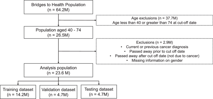
The population dataset from Bridges to Health (all those registered to a GP practice in England) is filtered to the age range of 40–74, and those with current and previous cancer diagnoses (relative to August 2021) are removed, resulting in an analysis dataset of 23.6M patients, which are then split into training, validation and testing datasets.
We use the period between August 2016 and August 2021 to construct our predictive features and patient histories. We then use these features to predict a cancer diagnosis in the period after September 2021. Our results focus on a 1-year predictive window between September 2021 and August 2022.
A stylised version of a patient pathway diagnosed with cancer in year 6 is presented in Fig. 2. In order to maintain a consistent length of 5 years of patient history, we used a single cut-off date for our analysis, and randomly split the analysis population between training, validation and testing. In the Supplementary Information (SI) we show results predicting up to 2 years after the cut-off date. We also present results when an exclusion gap is introduced after the cut-off date, to ignore diagnoses which may have occurred immediately after the cut-off date. These results are presented in the SI in the ‘Exclusion Gap’ analysis section.

The figure shows a stylised patient pathway with various types of events recorded during the 5 (history) + 1 (predictive window) years we observe the patients.
An individual’s patient history includes not only demographic information, but also comorbidities diagnosed during the 5-year period (between 2016 and 2021), as well as information on symptoms reported to NHS 111 lines. Individuals calling NHS 111 lines are triaged by trained personnel and based on their reported symptoms are referred to the appropriate services for further care. These could include primary care (with varying degrees of urgency), Accident & Emergency Care (A&E), or community/dental services. The dataset captures detailed information on the symptoms individuals reported as well as the type of referral (if any) the advisor made. For our analysis, we match the data on symptoms reported based on the pseudonymised patient number to the rest of the patient’s health record coming from their interactions with secondary care.
To create our patient histories, we complement data from NHS 111 lines with two national datasets. First, we use data from the Bridges to Health Segmentation (B2H). The dataset includes information on all individuals registered with a general practice in England and has rich information on demographics going beyond standard characteristics such as age, ethnicity and sex to also include household level information on the socioeconomic status of the household the person belongs to (e.g. urban professional). Household type information draws from the Acorn dataset23. The B2H itself draws from a large number of specialised national datasets covering health records beyond secondary care to also include mental health services and specialised tertiary care services. Drawing from this information several flags are created capturing a wide range of long-term conditions (e.g. COPD, physical disability, Downs syndrome). In our analysis, we only exclude those with the cancer flag as we want to ensure that our model predicts first incidence of cancer rather than recurrent cancer. In total, we include 59 binary features capturing a wider range of conditions from the B2H dataset. A detailed list of conditions is provided in Supplementary Table 1.
Second, we use data from the Secondary Uses Service (SUS) datasets and Emergency Care Services Dataset (ECDS) which covers all appointments/admissions and attendances to hospital secondary care services in England24,25. These datasets allow us to create features capturing the type of appointment the person had (e.g. outpatient appointment) and the associated diagnosis based on ICD–10 and SNOMED codes.
Data on mortality allows us to monitor who may have passed away after the cut-off date for reasons other than cancer and exclude those individuals from our data. We also exclude individuals with a previous cancer diagnosis. More details on dataset construction are included in the ‘methods’ section.
Note that excluding those passing away after the cut-off date due to other (than cancer) reasons could potentially introduce some bias in the results. However, the alternative is not without risks. Specifically, keeping those passing away from other reasons in our sample and treating them as negative cases (i.e. not diagnosed with cancer) would require assuming that none of the people passing away for other reasons (e.g. due to an accident) would have gone to develop cancer later during our prediction horizon. Clearly, a strong assumption which in our view could negate the potential advantages of including these individuals in our analysis.
Model prediction
We trained several classification models to predict the probability of being diagnosed with cancer in the coming year (September 2021–August 2022). We selected the XGBoost model as our preferred specification based on comparisons in terms of performance with the other classifiers (see comparison of machine learning algorithms in SI). Given the very sharp class imbalance between cancer and non-cancer cases, we use under sampling in our training datasets to ensure an equal number of cancer and non-cancer cases. We verified that the under sampled training dataset accurately represented the general control population on demographic variables such as age, gender, ethnicity and levels of deprivation (see Supplementary Table 7).
We predict the risk of cancer diagnosis for the nine cancer sites selected for the reasons discussed earlier. We also report the results for a model trained to predict any cancer diagnosis. By “any cancer diagnosis” we mean all cancer sites (see Supplementary Table 2 for ICD-10 codes) and not only the 9 cancer sites mentioned above.
For each of these models, we report several performance metrics for all cancer specific models, with a threshold value of 0.5 to ensure a balance between sensitivity and specificity (see Table 1). Each model was trained separately as a binary classifier. The ovarian cancer model was trained and tested only on females.
The size of datasets used for training, validation and testing for each of the cancer types is presented in Supplementary Table 3, and descriptive statistics on the whole population, and for the cancer and control population for each cancer site are presented in Supplementary Tables 4 and 5.
Important features
We demonstrate our approach for cohort construction by using bladder cancer, one of the priority cancer sites as our test case. In Table 2, we present some descriptive statistics focusing on the comparisons between those diagnosed with bladder cancer during the 1-year predictive window and those who were not.
As expected, there are noticeable differences in terms of age and gender between those diagnosed with bladder cancer in year 6 and those who were not. Cancer cases are predominantly male and older, reflecting the well-established link between age and cancer incidence, as well as the fact that bladder cancer is more frequent among males. Beyond demographics, the number of 111 calls reporting cancer related symptoms, as well as the number of A&E attendances, are higher on average for those diagnosed with bladder cancer in year 6 compared to those who are not. In total the model was trained on 821 features (see Supplementary Table 1 for full list).
Both the number of calls to NHS 111 lines reporting cancer related symptoms, as well as number of A&E attendances, will end up being among the most useful features for model prediction, as we will see later.
In order to improve model accuracy and to inform our work on constructing higher risk cohorts, we select the most important features using two metrics, gain and Shapley (SHAP) values.
In Fig. 3a, we show the SHAP values for the top 20 features (our models include 821 features in total) – ordered based on the gain metric (the average gain across all splits where the feature is used) for the XGBoost model (Fig. 3b). The red colour indicates higher values for the selected feature, and a positive SHAP value means an increase in the risk of cancer. For example, higher age has overwhelmingly positive SHAP values, which means that higher age is predicting higher risk of bladder cancer in the next year. By comparison, we show the mean absolute SHAP value for these features (Fig. 3c). While there are slight differences in the ordering of the most informative features, 17 out of the top 20 features based on average model gain are also amongst the top 20 features as determined by mean absolute SHAP value.

a SHAP value, shown by order of the top 20 features based on model gain value. Red (Blue) colour indicates high (low) values for the specific feature. Dots to the right (left) of the vertical line where SHAP value is zero indicate that this feature increases (decreases) predicted probability of cancer diagnosis in year 6. Features written in bold with an asterisk were also among the top 20 in feature importance based on mean absolute SHAP value. b XGBoost model average gain value c Mean absolute SHAP value for the top 20 features.
We observe that beyond age and gender, several comorbidities appear as relevant predictors of a bladder cancer diagnosis in ways that are consistent with expectations based on the medical literature. For example, the presence of chronic obstructive pulmonary disease (COPD) and urinary infections is associated with the incidence of bladder cancer in previous research26,27.
In addition, several features drawn from the NHS 111 calls dataset appear to be good predictors of bladder cancer incidence. For example, higher number of calls to NHS 111 lines reporting cancer related symptoms is one of the features with the highest gain metric value (just below demographics and long-term condition status). In addition, we also see that features capturing specific symptoms that are plausibly related to undiagnosed bladder cancer are also relevant and have the expected direction of effect. Specifically, higher number of calls to NHS 111 lines reporting “pain and frequency of passing urine” or “blood in urine” (during the last year) are both relevant predictors of risk of being diagnosed with bladder cancer in the next year.
To more comprehensively explore the importance of NHS 111 calls as predictors of risk of future cancer diagnosis, we replicated the analysis based on the gain metric for all other priority cancers beyond bladder. In all cases, features based on NHS 111 calls were among the most influential in predicting future cancer diagnosis. In Table 3, we report the rank of features, created from NHS 111 calls data, in terms of feature importance based on the gain metric. We do this for all cancer sites included in Table 1.
Table 3 highlights that features based on information captured in NHS 111 calls are among the top 20 features, based on the gain metric, and often among the top 5 or 10 for all cancer sites we explored in this study.
A comment regarding the predictive usefulness of symptoms reported in NHS 111 calls is warranted here. Some of the symptoms such as blood in urine may suggest that individuals would very quickly undergo medical evaluation which could lead to a relatively fast diagnosis of cancer. However, evidence from previous research on NHS 111 calls data suggests that a surprisingly high share of patients (close to one third) who are referred to urgent services such as emergency departments for a follow-up are actually not following the advice and neither appear to contact any other relevant health services following their call to NHS 11128. This means that it is very likely that many of the patients reporting what would appear as serious symptoms do not actually follow-up promptly thus postponing a potential diagnosis.
A possible concern with any analysis using patient histories is the possibility of data leakage. This could be the case if predictive features included in the analysis are indicative of a future cancer diagnosis in ways that undermine their predictive usefulness. For example, if a cancer diagnosis is recorded with a delay in the data, then it is conceivable that features strongly related with the diagnosis, such as cancer specific treatments, would “contaminate” the training data with the information about cancer diagnosis which we seek to predict. We however believe that this is unlikely to be the case here, for several reasons. First, our analysis excludes all those with a previous cancer diagnosis, and consequently also does not include treatments related to cancer as a predictive feature. Second, we do not include any cancer specific test results that could be construed as related to a future cancer diagnosis among our predictive features. Overall, the type of features we include such as demographics, symptoms reported in NHS 111 lines or comorbidities do seem much less likely to lead to such contamination as they are unlikely to be related to a yet not recorded diagnosis. Finally, we test our predictive models by excluding diagnoses in a time period after the cut-off date (see Exclusion Gap analysis in the SI) to confirm that our model can achieve good predictive performance even when focusing on cancers diagnosed more than 3 months after the cut-off date.
Constructing higher-risk cohorts
The primary goal for the analysis is to use the model results to construct high risk cohorts, for a cancer diagnosis within the next year, which can then be used to inform case finding and appropriate interventions to support earlier diagnosis and improve survival. We discuss two possible approaches to achieving this.
In the first, risk-based cohort construction method (Method A), we use the model risk probability at the individual patient level to create cohorts. Different sized cohorts can be constructed by varying the threshold for inclusion in the high-risk group.
The second feature-based cohort construction method (Method B) identifies cohorts with defined characteristics based on decision rules, utilising the most informative features from the trained model.
Method A: Risk based cohort construction
One approach to constructing higher risk cohorts is to consider capacity based on the requirements of a specific intervention/screening programme and then selecting the appropriate risk threshold which would lead to the desired cohort size. The risk thresholds are applied to the individual level predictions of the model. Based on different risk thresholds, higher risk cohorts of varying sizes can be constructed. The lower the risk threshold, the larger the size of the cohort, but the lower the potential incidence of cancer within the cohort. An illustration of this method is shown in Fig. 4.

Cohorts of different sizes are created by applying thresholds to model risk scores. The cancer incidence in such cohorts is calculated and compared to the baseline cancer rate to generate the lift value.
We define a lift value as the ratio of the cancer incidence within the cohort to the baseline cancer incidence. The baseline cancer incidence in our case, refers to those aged between 40–74 with no previous cancer diagnoses who go on to develop cancer in the next year. Based on different risk thresholds, one could construct a lift curve which plots the lift value against the size of the cohort on the x-axis.
An example based on the model on bladder cancer is provided in Fig. 5. The lift curve exhibits the expected shape where the lift value declines as we increase the size of the cohort. It also highlights the potential trade-off between high incidence and the total number of cancers correctly predicted. As the cohort size is increased, individuals with lower risk scores are included in the cohort, reducing the incidence and hence the lift value. The lift curve asymptotically approaches a lift value of 1—this represents the baseline cancer risk in the population (Fig. 5a).

Lift curve values for cohorts from a 0.5% to 100% of the population b 0.5% to 22% of the population. Predictions were obtained from a XGBoost model trained on all variables, and on another trained only on demographic variables to showcase the improved accuracy in identifying high risk groups when additional variables such as comorbidities and symptoms related to 111 calls are added.
Typically, the smaller the selected cohort of the population, the higher the lift value, as these are the individuals with the highest risk scores from the model. For example, in the top left of Fig. 5b, considering a cohort size of the highest risk (based on model probability risk score) 0.5% of the population (~125,000 individuals), the lift value of the model trained on all variables is 16, representing a cancer rate of 1 in 212 in the cohort. For a model trained on only demographic and socioeconomic variables (age, gender, ethnicity, IMD decile, integrated care board, acorn variables), the lift value for an equivalent cohort size is 9.4, representing a cancer rate of 1 in 357.
These values represent the potential order of magnitude improvement in cancer incidence in identifying high-risk cohorts using a risk score approach compared to chance selection from the population (cancer rate of 1 in 3355). If the cohort size is increased to the highest risk 5.8% of the population (~1.4 million individuals), the lift value reduces to 6.4 for the model with all variables (cancer rate 1 in 527) and 5.5 (cancer rate 1 in 613) for the model with demographic variables only. Lift curves for the other priority cancer sites are presented in Supplementary Fig. 4, and cohort cancer rates are presented in Supplementary Table 10.
These results also demonstrate the importance of including features from calls to NHS 111 lines, as well as comorbidities, to the model, as the resulting model risk scores can identify the highest risk individuals more accurately. As the cohort size increases, the difference in lift value between the two reduces, suggesting that both models capture the background demographic risk factors.
While more standard in terms of approach, Method A has several limitations from an operational perspective. First, Method A does not allow one to filter on features that may be most useful from a practical perspective. For example, depending on the type of intervention, one may want to focus on symptomatic patients and therefore select cohorts based on specific symptoms. Second, those charged with administering the interventions may not always have access to individual level predictions and instead would have to rely on flags drawing from specific features that are included in the data available to them. For example, eligibility for targeted lung health checks in England relies on age and smoking status.
This method also relies on applying thresholds to individual patient level predictions. While steps can be taken to explain the model (e.g. through feature importance and other techniques), ultimately the high-risk groups are a heterogeneous cohort. In Method B, we demonstrate how clearly defined cohorts can be created based on specific feature combinations.
A further limitation of this method is that the model may be biased towards predicting higher risk for certain demographic groups, making the high-risk cohort non representative of the actual incidence of bladder cancer in the population. As shown in the SHAP feature importance results (Fig. 3a), higher age, male, and white ethnicity all tend to increase the model risk score. This does correspond with higher incidence of bladder cancer in this group, however, given the low counts of bladder cancer among other demographic groups, it is difficult to ensure fair representation of all strata when constructing high-risk cohorts using this method, even when steps are taken to balance the training dataset. In the sub-group cohorts of Method B, we show how we sought to address this.
Method B: Feature based cohort construction
An alternative method that aims to overcome the above constraints is shown in Fig. 6 and outlined as follows. First, we select relevant features based on feature importance and data availability. The most important features, which were in the top 20 of model gain and SHAP value, were selected. SHAP was also used to identify the direction of the feature. Features which had a positive impact on the model output (i.e. which tended to increase the risk if the feature was present) were selected.

The most informative features from the trained model are identified and used to identify high-risk cohorts by identifying pairs of features which result in the cohorts with highest incidence. These decision rules can be applied either population wide, or to specific demographic sub-groups.
We then filter the population based on those features and examine the predicted cancer incidence. As is the case with Method A, we can then compare incidence of cancer in this curated cohort compared to the baseline incidence in the entire population.
This method has been applied to the whole population, and to sub-groups of demographic strata, demonstrating how the approach can be used for targeted interventions.
Population wide cohorts
The pair of features which would yield the highest incidence cohorts (on the validation data) of varying size (at least 10,000 to at least 250,000) were identified. Subsequently, the selected pair of features was applied to the test data to evaluate the expected bladder cancer incidence in the whole population. In Table 4, we show some examples of such curated cohorts based on combinations of just two features among those that the model considers as high importance for predicting cancer incidence in the next year. The cohort with highest cancer incidence, and a size of at least 10,000, is constructed based on interactions with the 111-call service and includes a specific bladder cancer related symptom of blood in urine. The cancer incidence within this cohort is 41 times higher than the overall incidence in the analysis population, with a cancer incidence of 1 in 82, compared to 1 in 3355 in the study population.
Larger cohorts of high-risk patients are constructed with flags relating to comorbidities of the genitourinary system and other diseases of the urinary system. Applying these flags to the population results in a cohort size of approximately 100,000 individuals, with a cancer rate 6 times higher than in the overall study population.
An example of a larger cohort of ~290,000 individuals would be constructed by applying the filter of patients having at least one long-term condition, and a diagnosis relating to symptoms and signs involving the genitourinary system in the last 5 years. This results in a cohort with a lift value of 4.5.
There is nothing in principle to prevent us from constructing cohorts based on combinations of more than two features (based on feature importance). Instead, our decision to opt for pairs of features is pragmatic. Especially when looking at population sub-groups based on gender/ethnicity (which we do in the next section) selecting more than two features would lead to very small cohorts, with sizes which are neither useful for practical purposes neither suitable for confidently inferring performance on the test dataset. As an example, the test dataset for the cohort of white males who had at least one call reporting cancer related symptoms in last year (AND) at least one call reporting blood in urine in last year (AND) have been diagnosed with hypertension includes just 517 individuals.
Sub-group cohorts
The population was segmented into demographic groups to investigate if different sets of features can create higher risk cohorts across demographic strata. This was also to address one of the limitations of method A, namely how we can ensure equality of opportunity if model predictions may be biased when there is insufficient training data from all demographic groups.
The segmentation was based on gender (male/female) and broad ethnicity (White/Non-white), resulting in four groups. Due to the low incidence of bladder cancer, more granular segmentation would have resulted in very small sample sizes.
For each population segment, the same methodology as described above was applied, with the cohort with the highest incidence of cancer cases being identified. These decision rules were then applied to the test dataset to evaluate the efficacy of the cohort. The lift value was calculated based on the incidence of cancer for each stratum. The results are shown in Table 5.
For the white ethnicity group, features related to 111 calls are particularly effective in identifying high risk groups. The specific nature of the symptom information (blood in urine) can result in small cohorts with lift values of 47.5 for white females, and 36 for white males.
In contrast, for the non-white ethnic group, more general health factors (e.g. A&E attendance) and comorbidities (e.g. COPD) result in the highest risk groups. These cohorts are still significantly higher in cancer incidence compared to baseline rates for these populations, as shown by the lift values of 2.9 for females, and 4.9 for males. However, they are also significantly lower than the lift values obtained for the white ethnic group. This potentially reflects health inequalities in the utilisation of services such as 111 calls. A key challenge here, which is not unique to our project, is the relatively fewer counts of cancer cases amongst the non-white ethnicities. For example, we observe only 97 instances of bladder cancer in the 1 year after the cut-off date in the non-white female population, compared to 4984 in the male white population. This presents the challenge of fewer samples to train the model on certain subgroups.
Discussion
This study makes several contributions to the burgeoning literature that seeks to use machine learning to develop useful predictive models for cancer incidence. First, our results demonstrate that information included in medical helplines such as NHS 111 calls contains useful signals predicting a future cancer diagnosis. Our is the first study that uses information on reported symptoms from medical helplines to predict a future cancer diagnosis. Our results, show that without exception for the nine cancer types we examined, features based on NHS 111 calls are among the most significant in terms of importance for predicting a future cancer diagnosis. While data quality and coverage are high when it comes to reported symptoms in NHS 111 calls, this dataset is not as comprehensive as primary care datasets. Future work should look to leverage those datasets alongside the information included in secondary care and NHS 111 calls to create a more complete patient history.
The second contribution of the study is to describe a practical method of constructing higher risk cohorts that could be tailored based on data availability, type of intervention, and desired levels of accuracy. We showcase this approach drawing from the model predictions for bladder cancer incidence. Beyond its greater flexibility, our approach also could mitigate the potential for bias due to the underrepresentation of certain demographic groups in the data.
Finally, ours is the first study employing multi-cancer prediction modelling using population level data from England. Our models exhibit good performance for most cancer types. These results further strengthen the case for using routinely collected national health data to stratify the population based on risk for future cancer incidence.
Our study is not without its limitations. For one, coverage of early reported symptoms of underlying disease is not as complete as it would have been if we had been able to use data from primary care. Second, predicting future cancer incidence does not differentiate based on stage of cancer diagnosis. It could be argued that predicting cohorts at risk of presenting at a late stage of cancer would be more valuable in terms of improving early diagnosis, as it could allow better targeting of those interventions to such populations. This information is available in the cancer registry database in England but was not available to the authors at the time of this research. Our study also does not include any information on lifestyle factors, which almost certainly play an important role in affecting the baseline risk of future cancer incidence. This is a limitation that is common in much of the previous work relying on secondary care data and this study is not going beyond previous research in that regard. Finally, while our approach to cohort construction can elucidate different risk factors that could be relevant for a variety of subgroups, it cannot ultimately overcome the limitations that stem from very low incidence among certain groups. As such, while absolute risk is always orders of magnitude higher than the baseline, relative accuracy is much more constrained for groups with very low incidence of the disease.
There are numerous potential practical applications of this analysis. Data could be used to inform case finding services for the high-risk cohorts identified. Such case finding services may be used to identify populations at a higher risk of developing cancer, who would benefit from ongoing surveillance, as well as individuals who may warrant an urgent diagnostic test for cancer. Populations with red flag symptoms of cancer, who meet referral thresholds indicated in NG12 (NICE guidelines on suspected cancer), could be triaged directly into urgent suspected cancer pathways29. Cohort characteristics could also be used to inform and better target opportunistic cancer checks, as well as local public awareness campaigns, reflecting symptom combinations and/or geographies with increased risk.
Our results for bladder cancer also suggest that the most informative high-risk cohorts cover symptomatic, rather than asymptomatic, patients. In that sense, our analysis is more directly relevant to interventions that seek to improve early diagnosis rates among those with symptoms that could be indicative of undiagnosed cancer rather than screening for asymptomatic patients.
More generally, considering previous research findings showing relatively low compliance with advice given in NHS 111 calls (e.g. among those advised to attend emergency services) and the fact that reported symptoms appear to strongly predict a future cancer diagnosis, interventions which would aim to increase compliance with triage advice may have considerable benefits in terms earlier diagnosis. More research is, however, required to better understand outcomes among those not following triage advice when it comes to cancer related symptoms. Exploring similar data sources in other settings could also help clarify the extent to which the type of symptom related signals we find in NHS 111 calls, in terms of future cancer diagnosis, are also relevant in other countries or useful for conditions beyond cancer.
Methods
Datasets
Our predictive models are trained on a dataset that captures an individual’s previous interactions with the healthcare system, their comorbidities, as well as a rich set of socio-demographic information. To create these patient histories, we combine several large datasets including the National Bridges to Health Segmentation Dataset, Secondary Use Services (SUS) data, ECDS, NHS 111 calls data, as well as ONS mortality data. A brief description of these datasets is provided below.
The National Bridges to Health Segmentation Dataset (B2H), which draws on a large number of datasets, provides information on long-term conditions for all patients, over 60 million, registered with General Practices in England30. In addition, we use the information included in B2H for socio-demographic characteristics (e.g. including race, age, sex, deprivation, household type) that could affect the risk of a future cancer diagnosis.
To complement the information included in B2H, we draw on data from the SUS and ECDS datasets, which include information on all outpatient, inpatient and emergency attendances in hospitals in England. This allows us to capture information on the number of previous inpatients/outpatients and emergency attendances. Frequency of interactions with the health system could reflect attitudes towards one’s health, beyond capturing underlying healthcare needs. For this reason, we construct several features which capture separately the number of previous hospital admissions, outpatient appointments, and emergency attendances within different time periods in the past (e.g. last year, last 5 years).
The SUS/ECDS datasets also allow us to capture detailed comorbidities as diagnosed in secondary care. We use ICD-10 codes covering 263 groups of comorbidities. ICD-10 codes are also used to construct the cancer diagnosis target flags (e.g. bladder cancer diagnosis in the next 52 weeks after the cut-off date). Supplementary Table 2 lists the ICD-10 codes used to identify the nine priority cancer sites, and for identifying any cancer (C00-C97, excluding C44).
A key dataset used in the analysis is the NHS 111 calls dataset. This dataset covers all calls made to NHS 111 lines between 2018–2023. It includes information on the symptoms the caller reported, as well as the date of the call. With the help of clinicians, we identified symptoms which may be related to cancer and constructed the relevant features capturing both the frequency of any cancer related symptoms reported, as well as the frequency for specific symptoms (e.g. blood in urine). Table 6 lists the cancer related symptoms.
Finally, to account for censoring due to death, we use person level data from the Office for National Statistics (ONS) death on mortality to capture those passing away during the period.
The various datasets are linked together using the pseudonymised ID that is common across the datasets. This allows us to create patient histories that capture all patient interactions with secondary care in the NHS, as well as any calls to the NHS 111 lines. Alongside any diagnosed comorbidities and sociodemographic information, this dataset provides rich information on which to build our predictive modelling.
Feature construction and preprocessing
In the section below, we describe in more detail how the features are constructed. We aimed to include a breadth of features capturing comorbidity, socio-demographic, geographic, symptom and healthcare system interactions. The complete variable list of features is listed in Supplementary Table 1. Predictive features were constructed for the period of the patient history (2016–2021) until the cut-off date of 31st August 2021. Cancer flags were constructed for the period after the cut-off date, identifying cancer diagnoses that occurred up to 2 years after the cut-off date.
Comorbidity
For each ICD-10 category 3 code block (e.g. A00-A09, A15-A19 … Z80-Z99), we create a flag per patient, to indicate if they received a diagnosis in this category, in the last year or last 5 years relative to the cut-off date. This was done by evaluating all diagnosis fields from SUS Inpatient, outpatient, A&E, and the ECDS.
Interactions with the healthcare system
The number of attendances at A&E, inpatient, and outpatient settings was calculated for each patient in the last year and the last 5 years from the cut-off date. The number of calls to 111 in the last year, and the number of calls with potentially cancer related symptoms was calculated.
Socio-demographic
We use one-hot encoding for categorical variables (Ethnicity, Index of multiple deprivation, Integrated Care Board, Acorn household type). The latter variables segment households into 6 categories (and 62 types) capturing financial circumstances, benefit receipt, health, wellbeing, and leisure and shopping behaviours. In addition, we include age, as well as an indicator variable capturing whether the individual is residing in a care home. For modelling purposes, we also impose several exclusions which we discuss below.
Exclusions and missing data
Our starting population is all individuals in England who are registered to a GP practice (the Bridges to Health Population). The focus of this analysis is individuals who are aged between 40 and 74 at the cut-off date between the observation and prediction window. We therefore exclude younger cohorts who are likely to have a much lower risk of developing cancer, as well as older individuals as shown in the data flow diagram in Fig. 1.
We then impose the following restrictions: we exclude those with a previous cancer diagnosis, as our focus here is on first diagnosis of cancer. We also exclude those who passed away before the cut-off date as well as those who passed away for any other reason than cancer after the cut-off date. We finally exclude the small number of individuals (1824) with missing information on gender.
Where data was missing for categorical variables, the null value was replaced with an ‘unknown’ string value. For those with missing data on ethnicity, we create an “unknown” flag and include this in the analysis.
Machine learning analysis
The dataset was split into train (60%), validation (20%), and test (20%) datasets through a random split. We performed a series of statistical tests to examine whether there were still systematic differences between the datasets in terms of demographics. No differences were observed between the datasets (details are included in Supplementary Table 6). The size of the datasets is shown in Supplementary Table 3.
For training models, the train dataset was randomly under sampled to ensure an equal number of cancer and non-cancer cases. This was done to avoid the issues stemming from large class imbalance due to the very small incidence of cancer in the data. We verified that the under sampled training dataset accurately represented the general control population on demographic variables such as age, gender, ethnicity and levels of deprivation (see Supplementary Table 7).
We trained four machine learning models: logistic regression, multilayer perceptron, random forest, and XGBoost. Hyperparameter optimisation was performed by optimising the receiver operating curve area under the curve, using the train and validation datasets with the hyperopt package. The hyperparameters and the ranges for optimisation are provided in Supplementary Table 8. We report model performance using the test dataset. XGBoost appears to perform better compared to the alternatives (see comparison of machine learning algorithms in SI—Supplementary Table 9, Supplementary Figs. 2 and 3), a fact consistent with its reputation in terms of performance when it comes to tabular data31.
Analysis was performed using python 3.10 on a spark cluster (3.5.0). Versions of the key packages used in the analysis are described in Supplementary Table 12.
Training features
The XGBoost model was trained with all features (Supplementary Table 1) and also with only demographic and socio-economic variables: age, gender, ethnicity, index of multiple deprivation, geographical variable (Integrated Care Board), care home flag, and acorn household type in order to explore the impact of features relating to 111 calls, comorbidities, and healthcare interactions on the model performance and high-risk cohorts.
Feature importance
Model feature importance was obtained from the XGBoost model by ranking features by their average gain across all splits the feature is used in. SHAP values were calculated on the validation dataset from trained models. SHAP calculates the contribution of each variable to the model predicted probability output32.
Method A: Risk based cohort construction
Individual patient level predictions were obtained on the test dataset. High-risk cohorts were constructed by varying the risk threshold and evaluating the cancer incidence within the cohort.
The cohort size (as shown in the lift curve in Fig. 5) was obtained by extrapolating to the whole population from the test dataset (which is a random sample comprising 20% of the whole study population).
Method B: Feature based cohort construction
The top 20 most informative features from model gain and SHAP were identified. Features which were present in both lists, and which tended to increase the risk if the feature was present, were selected. Demographic (gender and ethnicity) features were not selected as they were used to segment the population in the sub-group cohorts.
Each pair of selected features was used to filter the validation dataset. The size and incidence in the resulting cohort were calculated. For a particular cohort size, the combination of features which resulted in the highest cancer incidence was identified. This pairing of features was then applied to the unseen hold out test dataset to calculate the expected cancer incidence in the wider population. The cohort size in the whole study population was obtained by extrapolating from the test dataset.
For sub-groups, the same process as above was applied, with the difference that an additional filtering of the data by demographic strata was also applied.
Ethical approval
Not applicable. Data is collected and used in line with NHS England’s purposes as required under the statutory duties outlined in the NHS Act 2006 and Health and Social Care Act 2012. Data is processed using best practice methodology underpinned by a Data Processing Agreement between NHS England and Outcomes Based Healthcare Ltd (OBH), who produce the Segmentation Dataset on behalf of NHS England. This ensures controlled access by appropriate approved individuals, to anonymised/pseudonymised data held on secure data environments entirely within the NHS England infrastructure. Data is processed for specific purposes only, including operational functions, service evaluation, and service improvement. Where OBH has processed data, this has been agreed and is detailed in a Data Processing Agreement. The data used to produce this analysis has been disseminated to NHS England under Directions issued under Section 254 of the Health and Social Care Act 2012.
Data availability
All data used in this study are held internally by NHS England. The data cannot be shared publicly as they contain patient level sensitive information.
Code availability
Link to data processing notebook: https://github.com/nhsengland/cancer_foundry_data_modelling/. Code for data modelling available upon request from the authors. We plan to publish this code in the near future.
References
Appelbaum, L. et al. Development and validation of a pancreatic cancer risk model for the general population using electronic health records: an observational study. Eur. J. Cancer 143, 19–30 (2021).
Wang, Y. H., Nguyen, P. A., Mohaimenul Islam, M., Li, Y. C. & Yang, H. C. Development of deep learning algorithm for detection of colorectal cancer in EHR data. in Studies in Health Technology and Informatics Vol. 264, 438–441 (IOS Press, 2019).
Wang, X. et al. Prediction of the 1-year risk of incident lung cancer: prospective study using electronic health records from the state of Maine. J. Med. Internet Res. 21, e13260 (2019).
Hippisley-Cox, J. & Coupland, C. Development and validation of risk prediction algorithms to estimate future risk of common cancers in men and women: prospective cohort study. BMJ Open 5, e007825 (2015).
Malhotra, A., Rachet, B., Bonaventure, A., Pereira, S. P. & Woods, L. M. Can we screen for pancreatic cancer? Identifying a sub-population of patients at high risk of subsequent diagnosis using machine learning techniques applied to primary care data. PLoS ONE 16, e0251876 (2021).
Briggs, E. et al. Machine learning for risk prediction of oesophago-gastric cancer in primary care: comparison with existing risk-assessment tools. Cancers 14, 5023 (2022).
Ioannou, G. N. et al. Development of models estimating the risk of hepatocellular carcinoma after antiviral treatment for hepatitis C. J. Hepatol. 69, 1088–1098 (2018).
Ioannou, G. N. et al. Assessment of a deep learning model to predict hepatocellular carcinoma in patients with hepatitis C cirrhosis. JAMA Netw. Open 3, e2015626 (2020).
Howell, D. et al. Developing a risk prediction tool for lung cancer in Kent and Medway, England: cohort study using linked data. BJC Rep. 1, 1–11 (2023).
Zhen, J. et al. Development and validation of machine learning models for young-onset colorectal cancer risk stratification. NPJ Precis. Oncol. 8, 239 (2024).
Hippisley-Cox, J. & Coupland, C. A. Development and external validation of prediction algorithms to improve early diagnosis of cancer. Nat. Commun. 16, 3660 (2025).
Steinbuss, G. et al. Deep learning for the classification of non-Hodgkin lymphoma on histopathological images. Cancers 13, 2419 (2021).
Gaur, L., Bhandari, M., Razdan, T., Mallik, S. & Zhao, Z. Explanation-driven deep learning model for prediction of brain tumour status using MRI image data. Front. Genet. 13, 822666 (2022).
Fontanillas, P. et al. Disease risk scores for skin cancers. Nat. Commun. 12, 160 (2021).
Tammemägi, M. C. et al. Development and validation of a multivariable lung cancer risk prediction model that includes low-dose computed tomography screening results: a secondary analysis of data from the national lung screening trial. JAMA Netw. Open 2, e190204 (2019).
Varma, A. et al. Early prediction of prostate cancer risk in younger men using polygenic risk scores and electronic health records. Cancer Med 12, 379–386 (2023).
Placido, D. et al. A deep learning algorithm to predict risk of pancreatic cancer from disease trajectories. Nat. Med. 29, 1113–1122 (2023).
When to use NHS 111 online or call 111 - NHS. https://www.nhs.uk/nhs-services/urgent-and-emergency-care-services/when-to-use-111/.
Activity in the NHS | The King’s Fund. https://www.kingsfund.org.uk/insight-and-analysis/data-and-charts/NHS-activity-nutshell.
Beaulieu-Jones, B. K. et al. Machine learning for patient risk stratification: standing on, or looking over, the shoulders of clinicians? NPJ Digit. Med. 4, 1–6 (2021).
Williamson, A. E., McQueenie, R., Ellis, D. A., McConnachie, A. & Wilson, P. ‘Missingness’ in health care: associations between hospital utilization and missed appointments in general practice. a retrospective cohort study. PLoS ONE 16, e0253163 (2021).
Jung, A. W. et al. Multi-cancer risk stratification based on national health data: a retrospective modelling and validation study. Lancet Digit. Health 6, e396–e406 (2024).
Acorn consumer classification (CACI)—GOV.UK. https://www.gov.uk/government/statistics/quality-assurance-of-administrative-data-in-the-uk-house-price-index/acorn-consumer-classification-caci.
Emergency Care Data Set (ECDS)—NHS England Digital. https://digital.nhs.uk/data-and-information/data-collections-and-data-sets/data-sets/emergency-care-data-set-ecds.
Secondary Uses Service (SUS)—NHS England Digital. https://digital.nhs.uk/services/secondary-uses-service-sus.
Shephard, E. A. et al. Clinical features of bladder cancer in primary care. Br. J. Gen. Pract. 62, e598–e604 (2012).
Liao, S. et al. Associations between chronic obstructive pulmonary disease and ten common cancers: novel insights from Mendelian randomization analyses. BMC Cancer 24, 601 (2024).
Nakubulwa, M. A. et al. To what extent do callers follow the advice given by a non-emergency medical helpline (NHS 111): a retrospective cohort study. PLoS ONE 17, e0267052 (2022).
Overview | Suspected cancer: recognition and referral | Guidance | NICE. https://www.nice.org.uk/guidance/NG12/.
Valabhji, J. et al. Prevalence of multiple long-term conditions (multimorbidity) in England: a whole population study of over 60 million people. J. R. Soc. Med. 117, 104–117 (2024).
Borisov, V. et al. Deep neural networks and tabular data: a survey. IEEE Trans. Neural Netw. Learn. Syst. 35, 7499–7519 (2024).
Lundberg, S. M., Allen, P. G. & Lee, S.-I. A Unified Approach to Interpreting Model Predictions. https://github.com/slundberg/shap.
Acknowledgements
The authors would like to thank Robert Scott, and Thomas Henstock for their contributions in the scoping and analysis at the early stages of this study. We would also like to thank Michael Spence and Rajun Phagura for their help at various stages of the analysis. Finally, we are grateful to Anthony Cunliffe GP, Afsana Bhuyia GP, Tina George GP and Amelia Randle GP for sharing their clinical expertise.
Author information
Authors and Affiliations
Contributions
D.P. and H.M. contributed equally as co-first authors to this work. D.P. wrote the main manuscript text and contributed to the design of the analytical methodology. H.M. led on the design of the analytical methodology, contributed to the writing of the main text/supplementary material and to the analysis. D.B. led on the design of the analytical methodology, contributed to the writing of the main text and to the analysis. S.K. contributed to the analysis and to the writing of the main text/supplementary material. G.T., R.Ch., A.M. contributed to the scoping of the analysis, the design of the analytical methodology and manuscript revisions. R.Ca., E.H.W. contributed to the scoping of the analysis and the writing of the main manuscript. All authors have read and approved the manuscript.
Corresponding authors
Ethics declarations
Competing interests
The authors declare no competing interests.
Additional information
Publisher’s note Springer Nature remains neutral with regard to jurisdictional claims in published maps and institutional affiliations.
Supplementary information
Rights and permissions
Open Access This article is licensed under a Creative Commons Attribution-NonCommercial-NoDerivatives 4.0 International License, which permits any non-commercial use, sharing, distribution and reproduction in any medium or format, as long as you give appropriate credit to the original author(s) and the source, provide a link to the Creative Commons licence, and indicate if you modified the licensed material. You do not have permission under this licence to share adapted material derived from this article or parts of it. The images or other third party material in this article are included in the article’s Creative Commons licence, unless indicated otherwise in a credit line to the material. If material is not included in the article’s Creative Commons licence and your intended use is not permitted by statutory regulation or exceeds the permitted use, you will need to obtain permission directly from the copyright holder. To view a copy of this licence, visit http://creativecommons.org/licenses/by-nc-nd/4.0/.
About this article

Cite this article
Modarres, H., Pipinis, D., Balasubramanian, D. et al. Constructing multicancer risk cohorts using national data from medical helplines and secondary care. npj Digit. Med. 8, 551 (2025). https://doi.org/10.1038/s41746-025-01855-0
Received:
Accepted:
Published:
Version of record:
DOI: https://doi.org/10.1038/s41746-025-01855-0
