Multi-depot routing problem with van-based driverless vehicles

Abstract

In order to strengthen the coordination between different delivery participants and means of transport, this work proposes one extension of multi-depot routing problems where vans and driverless vehicles are used in combination during the delivery. The operation process mainly includes two parts. One is that, vans carry several driverless vehicles and goods, and drop off or pick up driverless vehicles at stops. Another is that, driverless vehicles departing directly from depots and dropped off by vans deliver goods to customers in cooperation. During the delivery, vans and driverless vehicles are in close cooperation through the proposed multi-depot joint distribution and the proposed van-van joint distribution. By the two modes, one van can depart from one depot and return to another depot, and one driverless vehicle can be set off by one van at one stop and be picked up by another van at another stop. This multi-depot routing problem with van-based driverless vehicles is formulated as a mixed integer programming model which can be solved by a designed heuristic algorithm. The sensitivity analyses about the maximum number of driverless vehicles in one van and the maximum traveling time of driverless vehicles are also performed. The results reveal that they have limited effects on the delivery cost and the application of the two modes. In addition, the experimental results demonstrate that the application of the two modes is affected by the distribution of depots and stops.

Introduction

Owing to urbanization and demographic growth, along with the increased diffusion of e-commerce, and new technologies, goods delivery in urban areas has developed widely^1,2. To make the delivery more efficient, the coordination between different delivery participants and means of transport should be strengthened. So multi-depot routing problem with van-based driverless vehicles (MDRP-VBDV) is introduced in this paper, based on multi-depot routing problem (MDRP) and the mothership concept that vans carry driverless vehicles (see Fig. 1).

Fig. 1

Van-based driverless vehicle. Source: Daimler, https://www.daimler.com/innovation/specials/future-transportation-vans/.

As e-commerce and home delivery services develop, logistic companies are pursuing more efficient delivery with a lower delivery cost. The cooperation between multiple depots can achieve the above aims, which leads to studies about MDRP³. Generally, MDRP involves routing a fleet of vehicles from several depots at minimal cost (e.g. distance) to serve some customers⁴. The cooperation degree between depots are different, which leads to MDRP with different characteristics, for example, the vehicle in use can return to the original depot or any depot including the original depot after delivery⁵. For MDRP where vans can depart from one depot and return to another depot, multiple scheduling later leads to the number of vans in each depot changed and some depots without vans. For the sustainability of the delivery system, the number of vans in each depot should remain unchanged at the beginning and ending of the delivery.

Due to the aging of the population and the development of the economy, labor costs are increasing⁶. With the acceleration of urbanization, problems such as traffic congestion, pollution and noise nuisance in cities are more and more serious. To deal with the above problems, lots of new technologies and innovative concepts for delivering goods are developed⁷. In this paper, goods delivery relies on driverless vehicle technology, which is summarized in detail by Jennings and Figliozzi⁸. Some studies have affirmed that driverless vehicle delivery will considerably reduce accidents, carbon emissions, and improve the convenience of people consuming⁹, while some logistics companies have tested and started driverless vehicle delivery, like JD.com, Meituan, and so on. In addition, public willingness to driverless vehicle delivery is researched by Milad et al.¹⁰ and Petri et al.¹¹. Limited by the technical level and relevant policies about driverless vehicles at this stage, it’s difficult for driverless vehicles to deliver goods independently¹². The mothership concept is that vans carrying driverless vehicles deliver goods to customers, which can improve the applicability of driverless vehicle delivery. Similar to the mothership concept, Mercedes-Benz Vans¹³ and Starship Technologies¹⁴ have cooperated in developing van-based delivery robots, and Starship Technologies is mainly responsible for providing autonomous robots during last-mile deliveries. Workhorse launched city delivery on the cooperation between trucks and drones¹⁵. Amazon is testing the airship with many small drones to complete last-mile delivery¹⁶. Boysen et al.¹⁷ and Yu et al.¹⁸ researched the van-based driverless vehicle delivery (VBDVD) in urban areas.

VBDVD has the following advantages:

(1) For security reasons, The speed of driverless vehicles is set to be slow¹⁹, which means that delivery with driverless vehicles only is inefficient. In addition, a large number of slow driverless vehicles may cause traffic congestion. VBDVD can avoid the above disadvantages of delivery with only driverless vehicles. (2) Compared with traditional delivery methods, VBDVD can greatly reduce the operational cost of logistics enterprises. Using driverless vehicles can reduce the labor cost. Moreover, driverless vehicles are powered by batteries, which can drastically reduce urban pollution. (3) For VBDVD, vans are equal to mobile depots, vans can drop off driverless vehicles and timely recover the broken down driverless vehicles during delivery. The number of stops where vans drop off or pick up driverless vehicles is always more than that of fixed depots, the scheduling plans of the former are more flexible. (4) Compared with van-based drone, VBDVD is more practical and safer in urban delivery. For example, drones are more susceptible to poor weather than driverless vehicles, and the environment where drones discharge goods is harsher than driverless vehicles²⁰. Moreover, drones can cause serious accidents in urban areas when breakdown.

Although VBDVD has been studied, the coordination between vans and driverless vehicles on the mothership concept needs to be strengthened further. In this paper, each van with several driverless vehicles and goods departs from a depot, then arrives at some stops in urban areas and drops off driverless vehicles^21,22. Driverless vehicles dropped off by one van deliver goods to customers and return to the nearest stop/depot after delivery. The returned driverless vehicles at stops can be picked up by any available van, which does not have to be the one dropped off them. After delivery, all dispatched vans and driverless vehicles return to depots. Note that the number of vans at each depot remains constant before and after the delivery. The number of driverless vehicles contained in each depot can be changed, driverless vehicles in each depot can be redistributed using other vehicles, which isn’t concluded in this paper.

The contributions of this paper are as follows. Based on MDRP and VBDVD, multi-depot routing problem with van-based driverless vehicles is introduced. To maintain the sustainability of the delivery system and improve the coordination of multiple depots, the multi-depot joint distribution is proposed, which is that the number of vans in each depot remains unchanged and vans can depart from one depot and return to another. To improve the coordination of driverless vehicles and vans on the mothership concept, the van-van join distribution is proposed, which is that driverless vehicles can be dropped off by one van at one stop and picked up by another van at other stops. Specifically, driverless vehicles directly departing from depots and dropped off by vans are scheduled for delivering goods in coordination. Later, this problem is formulated as a mixed integer programming model, and one heuristic algorithm to solve it is designed. Furthermore, we analyzed the influence of the maximum number of driverless vehicles in one van, and the maximum traveling time of driverless vehicles on scheduling plans.

The remainder of the paper is structured as follows. A brief literature review is provided in Sect. "Literature review". Then, Sect. "Problem description and model" describes the problem and the model. Section "Methodology" elaborates on the heuristic algorithm. A computational study is presented in Sect. "Computational study" and Sect. "Conclusion and future work" concludes the whole paper.

Literature review

MDRP-VBDV is a combinatorial optimization problem about delivering goods, which is similar to many variants of VRP. To describe MDRP-VBDV clearly, this section presents a literature review about MDRP and the mothership concept similar to VBDVD, we also distinguish MDRP/the mothership concept according to their characteristics and application. Later, we further explain the multi-depot joint distribution and the van-van joint distribution.

Multi-depot routing problem

Multi-depot routing problem is an extension of VRP. According to the cooperation degree of depots, whether the vans belong to depots and whether the delivery system is sustainable, there are mainly three types of multi-depot routing problems. The first is named fixed MDRP (F-MDRP)³, where each vehicle route must start and end at the same depot (see Fig. 2a). One popular approach to solve F-MDRP is to divide F-MDRP into several single-depot routing problems, which is a local optimization method and decreases the difficulty to compute. At the early stage, the approach is popularly used because each depot only serves customers in a fixed area, while no vans can deliver goods to customers in two different areas²³. For example, Laporte et al.²⁴ have developed one exact branch-and-bound algorithm for it, but the algorithm only works well for relatively small instances. Tillman and Hering²⁵, Golden et al.²⁶ and Raft²⁷ designed some heuristic algorithms based on simple construction and improvement procedures, the common solving strategy is to assign each customer to its nearest depot. Benoit et al.²³ proposed one tabu search algorithm combining the adaptative memory principle. But the approach reduces the flexibility of the delivery system. With the development of transportation infrastructure, people can travel between different areas frequently, which makes the customer demands in each area shift dynamically. The prominent disadvantage of this approach is that sometimes some depots need to serve many customers and other depots only need to serve several customers²⁸.

Fig. 2

Three types of multi-depot routing problems.

The second is named as multi-depot open routing problem (MDORP), where each vehicle departs from one depot and needn’t return to any depot after delivery (see Fig. 2b). MDORP is found quite frequently in practice. Due to many companies do not have their own fleet of vehicles for delivering goods or their own vehicles can’t meet delivering goods, MDORP arises, resulting in the need to rent some external vehicles²⁹. MDORP also occurs in other transportation problems, like school bus routing, taxi routing²⁹, and so on. Bae et al.³⁰ solved MDORP with time windows, with the objective to minimize the total delivery cost. Brandao³¹ proposed a memory-based iterated local search algorithm to solve MDORP.

The last is that the vehicle route can start at one depot and end at another. Due to the scarcity of relevant studies, we name this case as the multi-depot joint distribution. Limited to time windows of depots, distribution of customers and capacity of vehicles, the customers served by one vehicle (for the lowest delivery cost) aren’t in the obvious clustering character in terms of space. This means, vehicle routes around one depot may not lead to the lowest delivery cost and vehicle routes between two different depots can lead to the lowest delivery cost. Moreover, to maintain the sustainability of the delivery system, the number of vans in each depot should remain unchanged at the beginning and ending of delivery in this paper (see Fig. 2c). Otherwise, the allocation of vans at each depot will be imbalanced.

The mothership concept

The mothership concept firstly appeared in military and environmental monitoring³², that is later applied in delivering goods. Recently, there are mainly two methods of delivering goods on the mothership concept. One is van-based drone delivery (VBDD), which has been widely tested by companies like MecedesBenz and Matternet, and also by UPS and Workhorse, among others³³. Multiple van-based drone delivery modes have been proposed^34,35. Another is van-based driverless vehicle delivery (VBDVD), which is recently concerned^36,37. Compared with drones, driverless vehicles have more loading capacity, longer duration and safer operating conditions³⁸, resulting in better applicability of VBDVD than VBDD in urban delivery.

According to different stops where vans drop off or pick up drones/driverless vehicles, there are two cases for VBDD and VBDVD. One is that the stops are customers’ positions, in this case, vans can directly deliver goods to customers and drop off or pick up drones/driverless vehicles at the customers’ positions (see Fig. 3a–c). This case is mainly applied into VBDD because the customer’s demands may be more than the maximum loadings of drones. Another is that the stops are special positions, not the customers’ positions (see Fig. 3d–f). The case is mainly for VBDVD³⁴, because the special positions are more convenient for vans dropping off or picking up driverless vehicles and waiting. The latter is one variant of the location-routing problem³⁹.

Fig. 3

Six deliveries on the mothership concept.

According to different driverless vehicle/drone routes, there are three cases for VBDVD and VBDD. The first is that the ending stop and the starting stop in one driverless vehicle/drone route are the same (Fig. 3a and d). Driverless vehicles generally deliver goods at a low speed, which may lead to the much waiting time for vans. Because drones with high speed can reduce mostly the waiting time, there are many studies about VBDD applied into this case³⁴. Boysen et al.¹⁷ investigated an innovative last-mile concept, where autonomous robots are set off from vans to deliver goods to customers. To improve the delivery efficiency, some robot depots are located in urban areas. Vans can arrive at some stops and leave directly after setting off robots, later arrive at robot depots and supplement robots. After delivery, the robots return to robot depots. The computational study shows that the robot depots greatly contribute to an efficient delivery process, and the concept leads to a considerable waiting time for vans and fewer unsatisfied customers than the delivery without robot depots. But maintaining robot depots will lead to much cost.

The second is that the ending stop and the starting stop in one driverless vehicle/drone route are different (Fig. 3b and e). Vans remove to other stops for recovering driverless vehicles/drones instead of staying at one stop for driverless vehicles/drones returning, which improves van service efficiency. For VBDD with this characteristic, one case is that the vans only serve as mobile platforms for launching and recovering the drone, as shown in Fig. 3e. Alena et al.⁴⁰ designed hybrid truck-drone delivery, the drone can take off from the roof of the truck to deliver goods to customers. After the delivery, the drone flies back and lands on the roof of the truck. Another case is that vans also serve customers^{41,42,43,44,45}, as shown in Fig. 3b. For VBDVD with this characteristic, Yu et al.¹⁸ investigated an innovative two-echelon urban delivery problem. It’s special that one heuristic algorithm is designed and the speeds of driverless vehicles and vans are analyzed. There are main two shortages for this paper. Firstly, all goods are loaded into the driverless vehicles rather than vans in advance, which leads to more electricity consumption of driverless vehicles due to more loadings and more possible loss costs, for example, goods are stolen. Secondly, last-mile delivery is only implemented by driverless vehicles dropped off by vans, the driverless vehicles departing directly from depots aren’t considered, which isn’t suitable for the general delivery problem with customers around depots.

The last is that the ending stop and the starting stop in one driverless vehicle/drone route are in two different van routes (Fig. 3c and f). We name this case the van-van joint distribution. For VBDD with this characteristic, Wang et al.³⁴ developed a branch-and-price algorithm to solve it, but the van is only paired with on drone and the drone can only deliver goods to one or two customers once. Compared with drones, the maximum traveling time and the maximum capacity of driverless vehicles are larger, which makes the customers served by one driverless vehicle (for the lowest delivery cost) more widely distributed. The van-van joint distribution applied into VBDVD can lead to more combination schemes, which may lead to the lower delivery cost. There have been no studies about the van-van joint distribution applied into VBDVD. Some studies related to the mothership concept are summarized in Table 1.

Table 1 Some studies related to the mothership concept.

Problem description and model

Problem statement

The above literature reviews show that various problems about MDRP and the mothership concept have been researched. These problems are with different characteristics, especially for VBDVD. To build the model of MDRP-VBDV clearly, the characteristics of MDRP-VBDV in this paper are as follows.

• (i) There are multiple depots where a homogeneous fleet of vans and driverless vehicles is available. The number of vans and driverless vehicles in depots is sufficient.

• (ii) Vans can’t directly deliver goods to customers because vans for last-mile delivery are sensitively affected by traffic congestion. The driverless vehicles directly departing from depots and dropped off by vans perform last-mile delivery.

• (iii) Driverless vehicle routes are classified into six types. The first is that driverless vehicles depart from and return to one depot (see condition 1 in Fig. 4). The second is that driverless vehicles depart from one stop and return to one depot (see condition 2 in Fig. 4), the driverless vehicles are dropped off by vans at the stop. The third is that driverless vehicles depart from and return to one stop (see condition 3 in Fig. 4). The fourth is that driverless vehicles depart from one depot and return to one stop (see condition 4 in Fig. 4), the driverless vehicles are picked up by vans at the stop. The fifth is that driverless vehicles depart from one stop and return to another stop (see condition 5 in Fig. 4), two stops are in one driverless vehicle route. The sixth is that driverless vehicles depart from one stop and return to another stop (see condition 6 in Fig. 4), two stops are in different van routes.

• (iv) There are two independent spaces in each van for driverless vehicles and goods. One van paired with a fixed number of driverless vehicles and some goods departs from one depot.

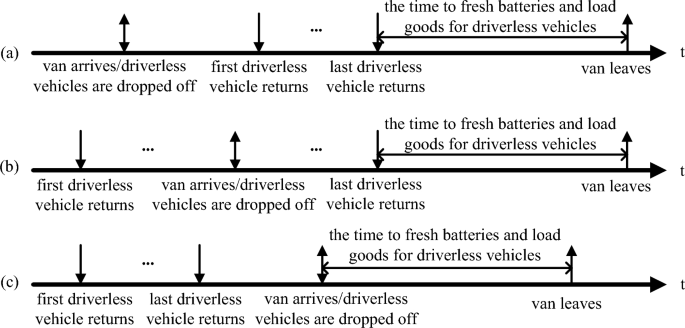
• (v) Driverless vehicles are dropped off at once when one van arrives at one stop, and dropping off driverless vehicles at other time isn’t considered. Later, some driverless vehicles intermittently return to the stop. After the last driverless vehicle returns, the batteries of the driverless vehicles are replaced together, and some driverless vehicles which can be dispatched at the next stop are loaded with goods. Lastly, vans depart from the stop for the next stop/depot. All operations at stops along time are shown in Fig. 5.

Fig. 4

Six types of driverless vehicle routes.

Fig. 5

Three cases for operations at stops along time.

Mixed integer programming model

For MDRP-VBDV, the objective is to minimize delivery cost, which contains the fixed cost and the transportation cost. The fixed cost is mostly determined by the number of drivers, one van is paired with one driver and the fixed cost is set to relate to the number of vans in this paper. The transportation cost is mainly determined by vehicle depreciation and electricity/fuel consumption, the transportation cost is set to relate to the distance that vans and driverless vehicles run in this paper.

All notations are shown in Table 2. Ensure that intermediate variables meet the corresponding constraints and decision variables are determined.

$${\text{min}}\left( {\sum\limits_{k \in K} {\sum\limits_{{i \in V_{0} }} {\sum\limits_{{j \in V_{1} }} {c_{1} x_{kij} } } } + \sum\limits_{k \in K} {\sum\limits_{{i \in V_{0} \cup V_{1} }} {\sum\limits_{{j \in V_{0} \cup V_{1} }} {c_{2} x_{kij} l_{ij} } } } + \sum\limits_{r \in R} {\sum\limits_{i \in V} {\sum\limits_{j \in V} {c_{3} x_{rij} l_{ij} } } } } \right).$$

(1)

Table 2 Notations.

The objective function is described by Eq. (1). The objective function (1) minimizes the delivery cost, which contains the fixed cost of vans and the transportation cost of vans and driverless vehicles.

$$\sum\limits_{k \in K} {\sum\limits_{{i \in V_{1} }} {x_{kij} } } = \sum\limits_{k \in K} {\sum\limits_{{h \in V_{1} }} {x_{kjh} } } , \, \forall j \in V_{0} .$$

(2)

Constraint (2) assures the number of vans at each depot remains unchanged after and before the delivery.

$$\sum\limits_{{i \in V_{0} }} {\sum\limits_{{j \in V_{{1}} }} {x_{kij} } } \le 1, \, \forall k \in K.$$

(3)

Constraint (3) implies that each van is dispatched no more than once.

$$\sum\limits_{k \in K} {\sum\limits_{{i \in V_{0} \cup V_{1} }} {x_{kij} } } = \sum\limits_{k \in K} {\sum\limits_{{h \in V_{0} \cup V_{1} }} {x_{kjh} } } , \, \forall j \in V_{1}$$

(4)

Constraint (4) indicates the number of vans arriving at one stop is equal to that departing from the stop.

$$\sum\limits_{k \in K} {\sum\limits_{{i \in V_{0} \cup V_{1} }} {x_{kij} } } \le 1, \, \forall j \in V_{1}$$

(5)

Constraint (5) indicates that one stop can be only visited no more than once by vans.

$$\sum\limits_{k \in K} {\sum\limits_{r \in R} {\sum\limits_{{i \in V_{0} }} {\sum\limits_{{j \in V_{1} }} {x_{krij} } } } } + \sum\limits_{r \in R} {\sum\limits_{{i \in V_{0} }} {\sum\limits_{{j \in V_{2} }} {x_{rij} } } } = \sum\limits_{k \in K} {\sum\limits_{r \in R} {\sum\limits_{{j \in V_{1} }} {\sum\limits_{{h \in V_{0} }} {x_{krjh} } } } } + \sum\limits_{r \in R} {\sum\limits_{{j \in V_{2} }} {\sum\limits_{{h \in V_{0} }} {x_{rjh} } } } .$$

(6)

Constraint (6) assures all driverless vehicles dispatched return to the depots after the delivery.

$$\sum\limits_{k \in K} {\sum\limits_{r \in R} {\sum\limits_{{i \in V_{0} \cup V_{1} }} {x_{krij} } } } + \sum\limits_{r \in R} {\sum\limits_{{i \in V_{2} }} {x_{rij} } } = \sum\limits_{k \in K} {\sum\limits_{r \in R} {\sum\limits_{{h \in V_{0} \cup V_{1} }} {x_{krjh} } } } + \sum\limits_{r \in R} {\sum\limits_{{h \in V_{2} }} {x_{rjh} } } , \, \forall j \in V_{1} .$$

(7)

Constraint (7) assures the number of driverless vehicles arriving at one stop is equal to that departing from the stop.

$$\sum\limits_{r \in R} {\sum\limits_{i \in V} {x_{rij} } } = \sum\limits_{r \in R} {\sum\limits_{h \in V} {x_{rjh} } } , \, \forall j \in V_{2} .$$

(8)

Constraint (8) assures the number of driverless vehicles arriving at one customer is equal to that departing from the customer.

$$\sum\limits_{r \in R} {\sum\limits_{i \in V} {x_{rij} } } = 1, \, \forall j \in V_{2} .$$

(9)

Constraint (9) indicates that one customer must be only visited once by one driverless vehicle.

$$\sum\limits_{{h \in V_{2} }} {x_{rjh} } \le 1, \, \forall r \in R,j \in V_{1} .$$

(10)

Constraint (10) implies that each driverless vehicle is dispatched no more than once at one stop.

$$\sum\limits_{{i \in V_{0} \cup V_{1} }} {\sum\limits_{{j \in V_{0} \cup V_{1} }} {t_{kij} x_{kij} } } \le t_{k} , \, \forall k \in K.$$

(11)

Constraint (11) guarantees that the traveling time of vans can’t exceed the maximum traveling time.

$$t_{ri} + t_{rij} - t_{rj} \le 2t_{r} \left( {1 - x_{rij} } \right), \, \forall r \in R,i,j \in V,$$

(12)

$$t_{rj} \le t_{r} , \, \forall r \in R, \, i \in V.$$

(13)

Constraint (12) and (13) guarantee that the cumulative traveling time of driverless vehicles can’t exceed the maximum traveling time.

$$T_{i} + t_{kij} + t_{si} - T_{j} \le 2l_{0} \left( {1 - x_{kij} } \right), \, \forall k \in K,i \in V_{1} ,j \in V_{0} \cup V_{1} ,$$

(14)

$$T_{i} + t_{rij} + t_{si} - T_{j} \le 2l_{0} \left( {1 - x_{rij} } \right), \, \forall r \in R,i \in V_{2} ,j \in V,$$

(15)

$$T_{j} \le l_{0} , \, \forall j \in V_{0} .$$

(16)

Constraints (14)–(16) indicate that all vans and driverless vehicles should return to depots before the ending time.

$$\sum\limits_{r \in R} {x_{krij} } \le Q_{kR} , \, \forall k \in K,i,j \in V_{0} \cup V_{1} .$$

(17)

Constraint (17) guarantees that the number of driverless vehicles carried by one van can’t exceed the maximum number.

$$Q_{kij} - Q_{kjh} \ge - Q_{k} \left( {1 - x_{rij} } \right) - Q_{k} \left( {1 - x_{rjh} } \right), \, \forall r \in R,i,h \in V_{0} \cup V_{1} ,j \in V_{1} ,$$

(18)

$$Q_{kij} \le Q_{k} , \, \forall k \in K,i,j \in V_{0} \cup V_{1} .$$

(19)

Constraints (18) and (19) guarantee that goods carried by one van can’t exceed the maximum capacity of the van.

$$Q_{rij} - Q_{rjh} - d_{j} \ge - Q_{r} \left( {1 - x_{rij} } \right) - Q_{r} \left( {1 - x_{rjh} } \right), \, \forall r \in R,i,h \in V,j \in V_{2} ,$$

(20)

$$Q_{rij} \le Q_{r} , \, \forall r \in R,i,j \in V.$$

(21)

Constraints (20) and (21) guarantee that goods carried by one driverless vehicle can’t exceed the maximum capacity of the driverless vehicle.

$$x_{krij} \in \left\{ {0,1} \right\}, \, \forall k \in K,r \in R,i,j \in V_{0} \cup V_{1} ,$$

(22)

$$x_{kij} \in \left\{ {0,1} \right\}, \, \forall k \in K,i,j \in V_{0} \cup V_{1} ,$$

(23)

$$x_{rij} \in \left\{ {0,1} \right\}, \, \forall r \in R,i,j \in V.$$

(24)

Constraints (22)–(24) are the constraints on variables.

Methodology

MDRP-VBDV in this paper is about the cooperation between multiple depots, multiple vans and multiple driverless vehicles. The proposed multi-depot joint distribution and the proposed van-van joint distribution make solving MDRP-VBDV more difficult than solving those problems in Table 1. To balance the speed and the effectiveness of solving, this section introduces one heuristic algorithm for MDRP-VBDV. In Sect. "Construct primary solutions" the method to obtain primary solutions is proposed. In Sect. "Iterated optimization", the method to optimize iteratively is proposed.

Construct primary solutions

The general structure to construct primary solutions is shown in Algorithm 1. Let $S_{1}$ be the set of all customer nodes, let $S_{2}$ be the set of stops and depots, let $S_{3}$ be the complete driverless vehicle route set and let $S_{4}$ be the complete van route set. The procedure GetDropOff-StartCustomerNode and FollowingNodeSearch are repeated to construct multiple driverless vehicle routes until no customer nodes are left. Afterwards, the procedure ConnectionHeuristic is applied to construct multiple van routes for serving all driverless vehicle routes.

Algorithm 1

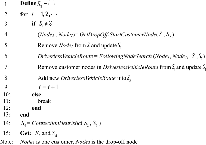
ConstructPrimarySolutions $\left( {S_{1} ,S_{2} } \right)$.

Constructing primary solutions is divided into two parts, one is to construct driverless vehicle routes (lines1-13) and another is to construct van routes (line14). The procedure GetDropOff-StartCustomerNode is to select the drop-off node (depot/stop) and the first customer node in one complete driverless vehicle route. In this paper, two strategies are used in GetDropOff-StartCustomerNode. One strategy is to select the drop-off node and the first customer node with the shortest distance¹². Another is shown in Algorithm 2, the analysis about parameter m is shown in Sect. “Analysis of the heuristic algorithm”. The two strategies are used to avoid infeasible combination (drop-off node and first customer) and maintain the diversity of solutions.

Algorithm 2

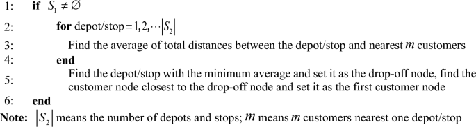
GetDropOff-StartCustomerNode $\left( {S_{1} ,S_{2} } \right)$.

After getting the drop-off node and the first customer node, we apply FollowingNodeSearch to select the following customers and the pick-up node (stop/depot) sequentially for constructing complete driverless vehicle routes. The nearest distance strategy and the random selection strategy are used in FollowingNodeSearch. Ensure the chosen nodes subject to all constraints. The constraints involve the time window of depots, the maximum capacity for goods and the maximum traveling time of driverless vehicles. The procedure FollowingNodeSearch is repeated until no customer node is left, finally, select the nearest stop or depot as the pick-up node to make a complete driverless vehicle route.

To construct complete van routes, we designed the procedure ConnectionHeuristic. The general structure of the procedure is sketched out in Algorithm 3. Let $S_{1}$ be the set of starting nodes and ending nodes of driverless vehicle routes, let $S_{2}$ be the set of all depots and $S_{3}$ be the set of van routes. The procedures GetStartDepotNode, GetVanRoute and ConnectionCheck are repeated to construct van routes until no nodes in $S_{1}$ are left.

Algorithm 3

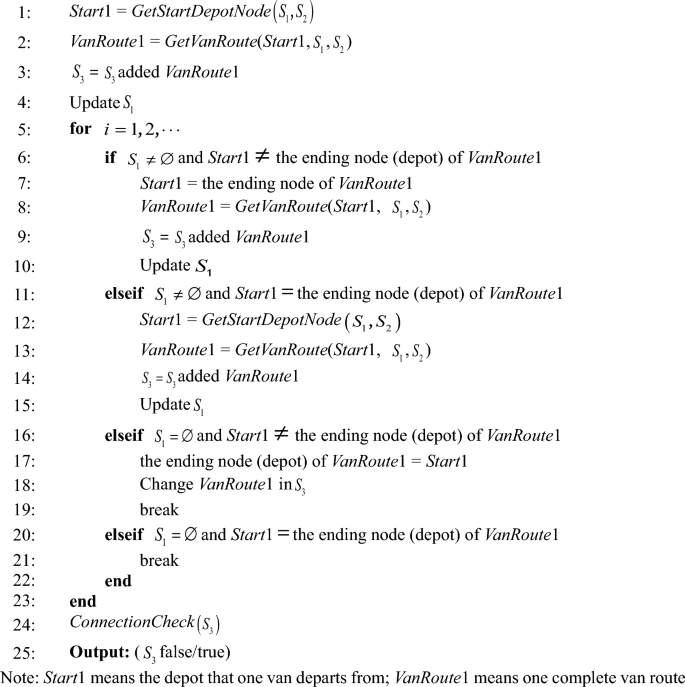
ConnectionHeuristic $\left( {S_{1} ,S_{2} } \right)$.

The procedure GetStartDepotNode in Algorithm 3 is applied to choose one depot as the starting node of one van route. GetStartDepotNode is based on the nearest distance criterion. The main steps are as follows.

• Step 1: remove all depots from set $S_{1}$ and update set $S_{1}$, which only contains stops.

• Step 2: remove duplicate stops from set $S_{1}$ and update set $S_{1}$.

• Step 3: run GetDropOff-StartCustomerNode $\left( {S_{1} ,S_{2} } \right)$, and the drop-off node is the starting node.

After ensuring the starting node of one van route, GetVanRoute is run to get one complete van route. Two strategies are used in GetVanRoute, one is the nearest distance criterion, and another is the shortest traveling time criterion, which thus yields a significant difference in initial solutions. Each van route should meet the constraints involving the maximum capacity of vans for goods, the maximum number of driverless vehicles in one van and the maximum traveling time of vans.

The procedure GetVanRoute is shown as follows. Considering the waiting time of vans at nodes, let the traveling time of each van route be much less than $t_{k}$ and the value $l_{0} - e_{0}$. So we introduce the parameter $z$ in line 2, and $z \in [0,1][0,1]$. Less value $z$ will lead to more vans in use and is convenient to construct feasible primary solutions, more value $z$ will lead to fewer vans in use and is difficult to construct feasible primary solutions.

Algorithm 4

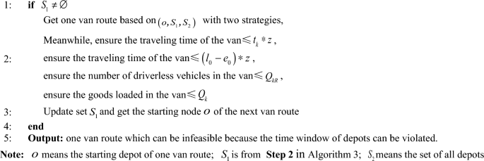
GetVanRoute $\left( {o,S_{1} ,S_{2} } \right)$.

In Algorithm 3, lines 6–22 ensure the number of vans at each depot unchanged. Lines 11–15 lead to unconnected loops rather than only connected loops, which increases the diversity of solutions. We give one example to explain above lines 11–15. The example contains depots A, B, C, D and stops 1, 2, 3, 4, 5, 6 (must be visited). Run the procedure GetStartDepotNode. If there is consideration for lines 11–15, the scheduling plan is shown in Fig. 6a, the first van route is A–1–2–B, the second van route is B–3–4–A and the third van route is D–5–6–D. If there is no consideration for lines 11–15, the scheduling plan is shown in Fig. 6b, the first van route is A–1–2–B, the second van route is B–3–4–A and the third van route is A–5–6–A. Two scheduling plans are different.

Fig. 6

The scheduling plans by two methods.

One driverless vehicle can be carried by different vans, so we can’t judge respectively whether one van route meets the time window of the depot. The procedure ConnectionCheck is aimed at judging whether the scheduling plans meet the time window of depots by introducing variable $w_{i}$,$w_{i}$ is the waiting time of one van at stop $i$. The scheduling plan meets the time window of depots, which means all waiting times of vans at stops exist. Figure 7 shows an example with constraints (25)–(30), where $\left[ {A_{0} ,A_{1} } \right]$ and $\left[ {B_{0} ,B_{1} } \right]$ respectively represent the time windows of depots A and B.

$$t_{A1k} + w_{1} + t_{12k} + w_{2} + t_{2Bk} \le B_{1} - A_{0}$$

(25)

$$t_{B3k} + w_{3} + t_{34k} + w_{4} + t_{4Ak} \le A_{1} - B_{0}$$

(26)

$$A_{0} + t_{A1k} + w_{1} \ge B_{0} + t_{B3k} + t_{31r}$$

(27)

$$B_{0} + t_{B31} + w_{3} \ge A_{0} + t_{A1k} + w_{1} + t_{12k} + t_{23r}$$

(28)

$$B_{0} + t_{B3k} + w_{3} + t_{34k} + w_{4} \ge A_{0} + t_{A1k} + t_{14r}$$

(29)

$$w_{2} = 0,\,\,\,w_{1} ,w_{3} ,w_{4} \ge 0$$

(30)

Fig. 7

An example to explain ConnectionCheck.

Constraints (25) and (26) ensure that each van travels in the time window of the depots. Constraints (27)–(29) make sure that the time when one van departs from one stop is after the time when all driverless vehicles return to the stop. For the stop where no driverless vehicle arrives, the waiting time is 0. For the example, the feasible solution ($w_{1}$,$w_{2}$,$w_{3}$,$w_{4}$) means that the scheduling plan (A–1–2–B, B–3–4–A, 1–4, 2–3, 3–1) meets the time windows of A and B.

Iterated optimization

We proposed one iterated neighborhood search approach with destroy and repair operators. The destroy and repair operators are mainly to reduce the number of vans in use for the primary solutions. The neighborhood search approach is mainly to reduce the total delivery cost during the whole iteration.

The structure of this designed heuristic algorithm is depicted in Fig. 8. To avoid local optimization and improve the quality of the final solution, the algorithm in this paper starts with multiple primary solutions^51,52,53. The value $A$ is set according to the actual problem. For example, we can get the distribution of the number of vans in use about the actual problem and set the average of this distribution as $A$. Acceptance criteria 1, 2 and 3 are the maximum iterated numbers in relative loops. The selected solutions in Fig. 8 can conclude feasible solutions and infeasible solutions. The main steps are as follows:

• Step 1: select the solutions where the number of vans in use is more than $A$ from multiple primary solutions and improve these solutions by the destroy and repair operators. Then let the improved solutions and other solutions go to step 2.

• Step 2: improve the solutions from step 1 by the neighborhood search operators and reserve the better solutions iteratively until meeting acceptance criteria 3.

Fig. 8

Heuristic flowchart.

Destroy and repair

To improve the efficiency of solving, not all primary solutions are dealt with neighborhood search operators directly. The solutions whose the number of vans in use is more than $A$, firstly need to be dealt with destroy and repair operators to reduce the number of vans in use. The destroy and repair operators in the paper include the insertion operator in condition② and the PD operators in “Neighborhood search”.

Neighborhood search

In this paper, we exploit general moves such as the insertion and the swap. Furthermore, the operators to change only pick-up nodes, change only drop-off nodes, change simultaneously drop-off nodes and pick-up nodes of driverless vehicle routes (PD operators) are also applied. The operators to change starting depots and ending depots of van routes (SE operators) are applied.

The insert operator is to remove one node and insert it at any nearby location, the swap operator is to swap one node with one nearby node. In this paper, the insert and swap operators are applied into two different scenes, one is in one driverless vehicle route and another is between different driverless vehicle routes. As shown in Fig. 9. Condition①: remove customer 1 and insert it after customer 3 in the driverless vehicle route 1. Condition③: swap customer 1 and customer 3 in the driverless vehicle route 1. Condition②: remove customer 3 in the driverless vehicle route 1 and insert it before customer 4 in the driverless vehicle route 2. Condition④: swap customer 3 in the driverless vehicle route 1 and customer 5 in the driverless vehicle route 2.

Fig. 9

Insert, swap and PD operators.

PD operators are shown as the conditions⑤–⑦. Condition⑤: change only the pick-up node of the driverless vehicle route 1. Condition⑥: change only the drop-off node of the driverless vehicle route 1. Condition⑦: change simultaneously the drop-off node and the pick-up node of the driverless vehicle route 1.

SE operators include three classes (replace, swap and 2-replace), as shown in Fig. 10. In condition⑧, SE operator is to replace one depot in use with another depot in use or not. In condition⑨, SE operator is to swap two depots in use. In condition⑩, SE operator is to replace two depots in use with other depots in use or not. In particular, the starting node and the ending node in connected loops are the same, which makes the number of vans at each depot unchanged.

Fig. 10

SE operators.

Computational study

Referring to the articles^17,54, we generated 27 types of instances with 2/3/4 depots and 9/11/13 stops and 15/30/50 customer nodes. Each type of instances is divided into 9 cases based on different serving time and different demands. All instances are solved by this designed heuristic algorithm many times. We analyze the effectiveness of this heuristic algorithm, implement the sensitivity analyses about the maximum number of driverless vehicles in one van and the maximum traveling time of driverless vehicles.

All computations are executed on a 64-bit PC with Core (TM) i7-7700 CPU under Windows 10. This heuristic algorithm is implemented using MATLAB (2016b).

Instance generation

Firstly, we generate a square with a side length 40 and the four vertices (0, 0), (0, 40), (40, 0) and (40, 40) are depots. To make all stops cover the most distribution area, the locations of thirteen stops are (10, 10), (10, 20), (10, 30), (20, 10), (20, 20), (20, 30), (30, 10), (30, 20), (30, 30), (20, 0), (0, 20), (20, 40) and (40, 20). All customers are located in the area randomly. The serving time and demand generation methods are as follows:

• Category A (CGA): randomly generate $t_{si}$ and $d_{i}$ of customer $i$,$t_{si} \in \left( {0,\,0.05t_{r} } \right)$,$d_{i} \in \left( {0,\,0.25Q_{r} } \right)$.

• Category B (CGB): randomly generate $t_{si}$ and $d_{i}$ of customer $i$,$t_{si} \in \left( {0.05t_{r} ,\,0.1t_{r} } \right)$ and $d_{i} \in \left( {0,\,0.25Q_{r} } \right)$.

• Category C (CGC): randomly generate $t_{si}$ and $d_{i}$ of customer $i$,$t_{si} \in \left( {0,\,0.1t_{r} } \right)$ and $d_{i} \in \left( {0,\,0.25Q_{r} } \right)$.

• Category D (CGD): randomly generate $t_{si}$ and $d_{i}$ of customer $i$,$t_{si} \in \left( {0,\,0.05t_{r} } \right)$ and $d_{i} \in \left( {0.25Q_{r} ,\,0.5Q_{r} } \right)$.

• Category E (CGE): randomly generate $t_{si}$ and $d_{i}$ of customer $i$,$t_{si} \in \left( {0.05t_{r} ,\,0.1t_{r} } \right)$ and $d_{i} \in \left( {0.25Q_{r} ,\,0.5Q_{r} } \right)$.

• Category F (CGF): randomly generate $t_{si}$ and $d_{i}$ of customer $i$,$t_{si} \in \left( {0,\,0.1t_{r} } \right)$ and $d_{i} \in \left( {0.25Q_{r} ,\,0.5Q_{r} } \right)$.

• Category G (CGG): randomly generate $t_{si}$ and $d_{i}$ of customer $i$,$t_{si} \in \left( {0,\,0.05t_{r} } \right)$ and $d_{i} \in \left( {0,\,0.5Q_{r} } \right)$.

• Category H (CGH): randomly generate $t_{si}$ and $d_{i}$ of customer $i$,$t_{si} \in \left( {0.05t_{r} ,\,0.1t_{r} } \right)$ and $d_{i} \in \left( {0,\,0.5Q_{r} } \right)$.

• Category I (CGI): randomly generate $t_{si}$ and $d_{i}$ of customer $i$,$t_{si} \in \left( {0,\,0.1t_{r} } \right)$ and $d_{i} \in \left( {0,\,0.5Q_{r} } \right)$.

According to related studies and actual applications, the other parameters is presented in Table 3. Assume that the traveling time of vans between two nodes is equal to the Euclidean distance between the two nodes, the traveling time of driverless vehicles between two nodes is five times more than that of vans between the two nodes. For example, the speed of vans is 60 km/h and that of driverless vehicles is 12 km/h. Sufficient vans and driverless vehicles are at each depot.

Table 3 The parameters.

Instances

To improve the speed of solving instances, different population sizes and iterations are set for different instances. In this paper, the population size is 200 and the iterations are 50 for the instances with 15 customers or 30 customers. The population size is 400 and the iterations are 300 for the instances with 50 customers.

This heuristic algorithm is run 5 times for each instance and the best solution is selected, as shown in Table 4.$M$ represents the delivery cost,$T$ represents the computation time. The first value of $R$ indicates the times of driverless vehicles dispatched on the van-van joint distribution (driverless vehicles travel between two stops in different van routes) and the second value indicates all times of driverless vehicles dispatched.$D$ represents the total traveling distance of vans and driverless vehicles. The first value of $V$ indicates the number of vans dispatched on the multi-depot joint distribution (vans travel between two different depots) and the second value indicates the total number of vans dispatched.

Table 4 The solutions for instances.

As shown in Fig. 11, the ratios in blue are the number of vans dispatched on the multi-depot joint distribution divided by the total number of vans dispatched, the ratios in red are the times of driverless vehicles dispatched on the van-van joint distribution divided by the total times of driverless vehicles dispatched. The ratios reflect the influence of the two modes on solutions. The larger the ratios are, the greater the influence of the two modes on solutions is. We don’t present the figure about instances with 15 customers because their ratios are all 0.

Fig. 11

The ratios for vans and driverless vehicles.

As shown in Table 4, the delivery cost decreases as the number of depots/stops increases. For example, the delivery cost of 9 instances with 4 depots/13 stops/50 customers is not more than those of 9 instances with 3depots/13stops/50customers, the delivery cost of 9 instances with 3depots/13stops/50customers is not more than those of 9 instances with 3depots/9stops/50customers.

As shown in Fig. 11, the ratios for vans are more than 0.3 and the ratios for driverless vehicles are more than 0.15, which indicates that the multi-depot joint distribution and the van-van joint distribution are influential on the solutions. For the small-scale instances with 15 customers, there is one van in each solution and the two modes don’t work. For instances with 30 customers and 50 customers, there are several vans in solutions and the multi-depot joint distribution and the van-van joint distribution can mostly reduce the delivery cost. Furthermore, the ratios for vans and driverless vehicles obviously change as the distribution of depots changes, and the ratios slightly change as the distribution of stops changes, as shown in Fig. 11. Which indicates that the influence of the two modes on solutions is affected by the distribution of depots and stops, some further analyses are shown in Sect. "Sensitivity analysis".

Analysis of the heuristic algorithm

In order to prove the effectiveness that this heuristic algorithm solves MDRP-VBD, we compare this heuristic algorithm with an adaptive genetic algorithm (IGA) which is proposed by Cho et al.⁵⁵, where the adaptive operator is to set dynamic genetic parameters. We also adopt multiple crossover operators (partial-mapped crossover, order crossover and order-based crossover) to improve IGA. Two algorithms are run 5 times for instances in Table 5 and the last 24 instances are from article²². $M$ represents the lowest delivery cost, $A$ represents the average delivery cost for 5 times, $T$ represents the average solving time for 5 times, $G$ represents the deviation between $A$ and $M$.

Table 5 The solutions of two algorithms.

Table 5 indicates that this designed algorithm is mostly better than IGA. $M$ and $A$ obtained by this designed algorithm are smaller than those by IGA, which indicates that this designed algorithm can solve instances in depth. For most instances, $G$ obtained by this designed algorithm is smaller than $G$ by IGA, which indicates that this algorithm can steadily solve instances. In addition, $T$ obtained by the designed algorithm is near to $T$ by IGA and less than 2 h, which indicates that this algorithm can be applicable to actual problems.$G$ of the front 18 instances is mostly larger than $G$ of the last 24 instances, because the distributions of customers, depots and stops are different.

In addition, we analyzed the method to construct primary solutions. Firstly, we analyzed the nearest distance strategy and the random strategy in FollowingNodeSearch. The instance 4depots/9stops/15customers-CGA is selected and respectively solved 10 times by this designed algorithm with the only nearest distance strategy, with the only random strategy, with the nearest distance strategy and the random strategy. As shown in Fig. 12, the maximum iterations are set to 30. Curves in red represent the convergence processes by the only random strategy and all curves in red distribute dispersedly. Curves in green represent the convergence processes by the only nearest distance strategy and all curves in green are mainly distributed above in Fig. 12, which indicates the only nearest distance strategy easily leads to local optimization. Curves in black represent the convergence processes by the nearest distance strategy and the random strategy, all curves in black are mainly distributed below in Fig. 12, which indicates using the third method in this paper can improve the efficiency of solving.

Fig. 12

The convergence processes under different strategies.

Next, we analyzed the influence of the value $m$(in algorithm 2) on the convergence processes. The instance 3depots/9stops/30customers-CGD is selected and solved 10 times under different value m, as shown in Fig. 13. The curve in blue represents the average number of accumulated iterations when the lowest delivery cost becomes 3500 during the convergence processes. The cure in orange represents the average number of accumulated iterations when the lowest delivery cost becomes 3200 during the convergence processes. From Fig. 13, we know that the convergence speed is fastest while $m$ is 3 or 4 and it slows down while $m$ is far away from 3 or 4. Actually, $m$ corresponds the the average number of customers served by one driverless vehicle at one time. Generally, we can’t in advance ensure the exact value m for solving delivery problems and we only can get some relatively effective values through data analysis.

Fig. 13

The number of iterations under different $m$.

Sensitivity analysis

Some instances in Sect. "Instance generation" are randomly selected and each instance is solved 10 times under different parameters ($Q_{kR}$ and $t_{r}$). The other parameters are from Table 3.

Firstly, the influence of $Q_{kR}$ on the delivery cost and the application of the two modes is analyzed. There are usually limitations for the loadings of vans on urban roads, meanwhile, the limited loadings of vans have to be divided into two parts for goods and driverless vehicles. Thus, we must explore the relationship between $Q_{kR}$ and the delivery cost, and reasonably allocate the loadings of vans for goods and driverless vehicles. In addition, the two modes are applied, which causes the calculating time to increase. Analyzing the influence of $Q_{kR}$ on the application of the two modes and determining whether to apply the two modes under different $Q_{kR}$ are necessary. The results are depicted in Table 6 and Fig. 14a–c.

Table 6 The delivery plans under different $Q_{kR}$.

Fig. 14

Delivery cost and the ratios for vans or driverless vehicles under different $Q_{kR}$.

Later, the influence of $t_{r}$ on the delivery cost and the application of the two modes is analyzed. Generally, big $t_{r}$ means that the batteries of driverless vehicles are more powerful and more expensive. We can choose suitable batteries by analyzing the relationship between $t_{r}$ and the delivery cost. The two modes reflect the cooperation between different depots and vans, we can know whether to strengthen the cooperation under different maximum traveling time of driverless vehicles. The results are depicted in Table 7 and Fig. 15a–e.

Table 7 The delivery plans under different $t_{r}$.

Fig. 15

Delivery costs, the ratios and the times of driverless vehicles under different $t_{r}$. (a) Delivery cost (b) The ratios for vans (c) The ratios for driverless vehicles (d) The times of driverless vehicles dispatched (e) The times of driverless vehicle dispatched on the van-van joint distribution.

As shown in Table 6, “—” represents no feasible solution. In Fig. 14a, we use one very big delivery cost “7000” to represent no feasible solution.$A$ represents the average delivery cost for 10 times. The first value of $V$ indicates the average number of vans dispatched on the multi-depot joint distribution, and the second value indicates the average number of vans dispatched. The first value of $R$ indicates the average times of driverless vehicles dispatched on the van-van joint distribution, and the second value indicates the average times of driverless vehicles dispatched.

As shown in Fig. 14a, the delivery cost of some instances always remains unchanged as $Q_{kR}$ changes. For other instances (4/9/30-CGF, 4/9/50-CGH, 4/13/50-CGD, 3/9/50-CGA and 3/13/50-CGB), the delivery cost firstly decreases and later remains unchanged as $Q_{kR}$ increases. It shows increasing the number of driverless vehicles in one van only causes a limited reduction of the delivery cost. Generally, when one van only carries a few driverless vehicles, it has to wait for long time until driverless vehicles arrive at stops, which reduces the number of customers that one van can serve and increases the number of vans dispatched. Of course, the maximum number of driverless vehicles in one van can’t be too large, two many driverless vehicles in one van can weaken the loadings for goods.

As shown in Fig. 14 b and c, the influence of the two modes on solutions is affected by $Q_{kR}$. The most ratios for vans in Fig. 14b are more than 0.3 and, the ratios for driverless vehicles in Fig. 14c are mainly in the interval (0.05, 0.4), which indicates that the multi-depot joint distribution and the van-van joint distribution are significantly influential on solutions, The bold and black value in Fig. 14b and c represents the average of all ratios for each group. For the instances with same stops and same customers, the more adequately the depots are distributed, the greater the influence of the multi-depot joint distribution on solutions is, as shown in Fig. 14b. The more inadequately the depots are distributed, the greater the influence of the van-van joint distribution on solutions is, as shown in Fig. 14c. For the instances with same depots and same customers, the more inadequately the stops are distributed, the greater the influence of the multi-depot joint distribution on solutions is, as shown in Fig. 14b. The more adequately the stops are distributed, the greater the influence of the van-van joint distribution on solutions is, as shown in Fig. 14c.

As shown in Fig. 15a, the delivery cost decreases when $t_{r}$ varies from 30 to 60 and remains unchanged when $t_{r}$ varies from 60 to 70. It shows increasing the maximum traveling time of driverless vehicles only causes a limited reduction of the delivery cost. For each instance, the maximum reduction of delivery cost is less than 500, which means that the reduction of delivery cost is only the transportation cost. As shown in Table 7, while $t_{r}$ approaches to the maximum traveling time of vans (80), the number of vans dispatched nearly is unchanged, which indicates that the delivery with vans and driverless vehicles is better than the delivery with only driverless vehicles. Limited to the maximum capacity of driverless vehicles and all depots are located in the suburbs, the transportation cost will be very much by only driverless vehicles. For example, there are many customers located at the center of the distribution area. All depots are located at the border of the distribution area, and driverless vehicles can deliver goods to several customers once. The transportation cost by only driverless vehicles traveling between the center of the distribution area and depots will be very much. For delivery where vans carry driverless vehicles, the vans are equal to mobile depots, which can reduce mostly the transportation cost of driverless vehicles. In addition, the speed of driverless vehicles is small, the delivery with only driverless vehicles is impractical⁵⁶.

As shown in Fig. 15b and c, the influence of the two modes on solutions is affected by $t_{r}$, the changing of the ratios for vans is irregular and the changing of the ratios for driverless vehicles is regular. In Fig. 15c, for most instances, the ratios for driverless vehicles increase when $t_{r}$ varies from 30 to 40, decrease when $t_{r}$ varies from 40 to 60 and remain almost unchanged when $t_{r}$ varies from 60 to 70. The changing of the ratios for driverless vehicles depends on the changing of total times of driverless vehicles dispatched and the changing of times of driverless vehicles dispatched on the van-van joint distribution. The total times of driverless vehicles dispatched decrease when $t_{r}$ varies from 30 to 60 and remain unchanged when $t_{r}$ varies from 60 to 70, as shown in Fig. 15d. The reason is that large value $t_{r}$ causes driverless vehicles can deliver more goods to more customers once (as shown in Figs. 16 and 17), which leads to fewer times of driverless vehicles being dispatched. The times of driverless vehicles dispatched on the van-van joint distribution mostly increase when $t_{r}$ varies from 30 to 40, decrease when $t_{r}$ varies from 40 to 60, and remain almost unchanged when $t_{r}$ varies from 60 to 70, as shown in Fig. 15e. The reason is that, at the beginning, large value $t_{r}$ causes driverless vehicles can travel between different stops, which leads to more times of driverless vehicles being dispatched on the van-van joint distribution. Later, large value $t_{r}$ causes many customers can be served by the driverless vehicles directly departing from depots instead of those on the van-van join distribution, which leads to fewer times of driverless vehicles being dispatched on the van-van joint distribution.

Fig. 16

The average loadings of driverless vehicles at one time under different $t_{r}$.

Fig. 17

The average traveling time of driverless vehicles at one time under different $t_{r}$.

Conclusion and future work

This paper introduces MDRP-VBDV, which contains vans and driverless vehicles delivering goods cooperatively, vans delivering on the multi-depot joint distribution and driverless vehicles delivering on the van-van joint distribution. In particular, to maintain the sustainability of the multi-depot joint distribution system, the number of vans at each depot should remain unchanged after and before the delivery. Driverless vehicles directly departing from depots and dropped off by vans deliver goods to customers cooperatively. The studies about MDRP-VBDV provided a reference for logistics enterprises.

In this paper, the mixed integer programming model of MDRP-VBDV is constructed and one heuristic algorithm for solving MDRP-VBDV is designed. The constraints contain the time windows of depots, the maximum capacity, the maximum traveling time, and so on. During generating primary solutions, the driverless vehicle routes are obtained first, and then the van routes. To ensure primary solutions be diversified, multiple strategies are applied into this algorithm. The performance evaluation about this algorithm under different strategies and different parameters is implemented. During iterated optimization, the destroy operators, the repair operators and multiple neighborhood search operators are adopted. Compared with the other traditional heuristic algorithm, this designed heuristic algorithm is better at solving MDRP-VBDV.

In addition, we implemented sensitivity analyses about the maximum number of driverless vehicles in one van and the maximum traveling time of driverless vehicles. We find that increasing the maximum number of driverless vehicles in one van or the maximum traveling time of driverless vehicles will only lead to a limited reduction in delivery cost. Selecting the suitable maximum number of driverless vehicles in one van and the suitable maximum traveling time of driverless vehicles is beneficial for the distribution problem. The influence of the two modes on delivery plans is affected by the above two factors. In particular, there is a regular relationship between the influence of the van-van join distribution on delivery plans and the maximum traveling time of driverless vehicles. By analyzing it, we can decide whether to apply the van-van joint distribution under different maximum traveling time of driverless vehicles. Moreover, the influence of the two modes on the delivery plan is affected by the distribution of depots and stops. We should also analyze the distribution of depots and stops before judging whether to implement the two modes.

Future research would focus on more efficient solving algorithms and considering EV charging stations. Most driverless vehicles are powered by batteries and considering EV charging stations can extend the maximum traveling time of driverless vehicles. So the research considering EV charging stations is more realistic and significant.

References

Liu, B., Guo, X., Yu, Y. & Zhou, Q. Minimizing the total completion time of an urban delivery problem with uncertain assembly time. Transp. Res. Part E Logist. Transp. Rev. 132, 163–182. https://doi.org/10.1016/j.tre.2019.11.002 (2019).
Perboli, G. & Rosano, M. Parcel delivery in urban areas: Opportunities and threats for the mix of traditional and green business models. Transp. Res. Part C Emerg. Technol. 99, 19–36. https://doi.org/10.1016/j.trc.2019.01.006 (2019).
Bekta, T., Luis, G. & Santos, D. Compact formulations for multi-depot routing problems: theoretical and computational comparisons. Comput. Oper. Res. 124, 105084. https://doi.org/10.1016/j.cor.2020.105084 (2020).
Lim, A. & Wang, F. Multi-depot vehicle routing problem: a one-stage approach. IEEE Trans. Autom. Sci. Eng. 2, 397–402. https://doi.org/10.1109/TASE.2005.853472 (2005).
Sadati, M. E. H., Aksen, D. & Aras, N. The r-interdiction selective multi-depot vehicle routing problem. Int. Trans. Oper. Res. 27, 835–866. https://doi.org/10.1111/itor.12669 (2020).
Anderluh, A., Hemmelmayr, V. C. & Nolz, P. C. Synchronizing vans and cargo bikes in a city distribution network. Cent. Eur. J. Oper. Res. 25, 345–376. https://doi.org/10.1007/s10100016-0441-z (2017).
Speranza, M. G. Trends in transportation and logistics. Eur. J. Oper. Res. 264, 830–836. https://doi.org/10.1016/j.ejor.2016.08.032 (2018).
Jennings, D. & Figliozzi, M. Study of sidewalk autonomous delivery robots and their potential impacts on freight efficiency and travel. Transp. Res. Rec. 2673, 317–326. https://doi.org/10.1177/0361198119849398 (2019).
Pettigrew, S. & Cronin, S. L. Stakeholder views on the social issues relating to the introduction of autonomous vehicles. Transp. Policy 81, 64–67. https://doi.org/10.1016/j.tranpol.2019.06.004 (2019).
Milad, G. & Akshay, V. The potential impact of media commentary and social influence on consumer preferences for driverless cars. Transp. Res. Part C Emerg. Technol. 127, 103132. https://doi.org/10.1016/j.trc.2021.103132 (2021).
Launonen, P., Salonen, A. O. & Liimatainen, H. Icy roads and urban environments. Passenger experiences in autonomous vehicles in Finland. Transp. Res. Part F Traffic Psychol. Behav. 80, 34–48. https://doi.org/10.1016/j.trf.2021.03.015 (2021).
Karmakar, G., Chowdhury, A., Das, R., Kamruzzaman, J. & Islam, S. Assessing trust level of a driverless car using deep learning. IEEE Trans. Intell. Transp. Syst. 22, 4457–4466. https://doi.org/10.1109/TITS.2021.3059261 (2021).
Ola, K. et al. Information on Daimler AG. https://www.daimler.com/innovation/specials/future-transportation-vans/paketbotes (2022).
Andrew J H. Thousands of autonomous delivery robots are about to descend on us college campuses. https://www.theverge.com/2019/8/20/20812184/starship-delivery-robot-expansion-college-campus (2019).
Stephen, B. Trucks carrying drones. https://www.360che.com/news/161115/70105.html (2016).
Zhao, Han. Qing. Amazon airship distribution. https://baijiahao.baidu.com/s?id=1629778680882933979&wfr=spider&for=pc (2019).
Nils, B., Stefan, S. & Felix, W. Scheduling last-mile deliveries with truck-based autonomous robots. Eur. J. Oper. Res. 271, 1085–1099. https://doi.org/10.1016/j.ejor.2018.05.058 (2018).
Yu, S. H., Jakob, P. & Sun, S. D. Two-echelon urban deliveries using autonomous vehicles. Transp. Res. Part E Logist. Transp. Rev. 141, 102018. https://doi.org/10.1016/j.tre.2020.102018 (2020).
Manuel, O., Andreas, H. & Alexander, H. The multi-vehicle truck-and-robot routing problem for last-mile delivery. Eur. J. Oper. Res. 310, 680–697. https://doi.org/10.1016/j.ejor.2023.03.031 (2023).
Zhang, N., Zhang, M. & Low, K. H. 3D path planning and real-time collision resolution of multirotor drone operations in complex urban low-altitude airspace. Transp. Res. Part C Emerg. Technol. 129, 103123. https://doi.org/10.1016/j.trc.2021.103123 (2021).
Liu, T., Luo, Z., Qin, H. & Lim, A. A branch-and-cut algorithm for the two-echelon capacitated vehicle routing problem with grouping constraints. Eur. J. Oper. Res. 266, 487–497. https://doi.org/10.1016/j.ejor.2017.10.017 (2018).
Dellaert, N., Dashty Saridarq, F., Van Woensel, T. & Crainic, T. G. Branch-and-price–based algorithms for the two-echelon vehicle routing problem with time windows. Transp. Sci. 53, 463–479. https://doi.org/10.1287/trsc.2018.0844 (2018).
Crevier, B., Cordeau, J. F. & Laporte, G. The multi-depot vehicle routing problem with inter-depot routes. Eur. J. Oper. Res. 176, 756–773. https://doi.org/10.1016/j.ejor.2005.08.015 (2007).
Laporte, G., Nobert, Y. & Arpin, D. An exact algorithm for solving a capacitated location-routing problem. Ann. Oper. Res. 6, 291–310. https://doi.org/10.1007/BF02023807 (1986).
Tillman, F. A. & Hering, R. W. A study of a look-ahead procedure for solving the multiterminal delivery problem. Transp. Res. 5, 225–229. https://doi.org/10.1016/0041-1647(71)90023-2 (1971).
Golden, B. L., Magnanti, T. L. & Nguyen, H. Q. Implementing vehicle routing algorithms. Networks 7, 113–148. https://doi.org/10.1002/net.3230070203 (1977).
Raft, O. M. A modular algorithm for an extended vehicle scheduling problem. Eur. J. Oper. Res. 11, 67–76. https://doi.org/10.1016/S0377-2217(82)80011-8 (1982).
Holland, C., Levis, J., Nuggehalli, R., Santilli, B. & Winters, J. Ups optimizes delivery routes. Interfaces 47, 8–23. https://doi.org/10.1287/inte.2016.0875 (2018).
Soto, M., Sevaux, M., Rossi, A. & Reinholz, A. Multiple neighborhood search, tabu search and ejection chains for the multi-depot open vehicle routing problem. Comput. Ind. Eng. 107, 211–222. https://doi.org/10.1016/j.cie.2017.03.022 (2017).
Bae, H. & Ilkyeong, M. Multi-depot vehicle routing problem with time windows considering delivery and installation vehicles. Appl. Math. Model. 40, 6536–6549. https://doi.org/10.1016/j.apm.2016.01.059 (2016).
Brando, J. A memory-based iterated local search algorithm for the multi-depot open vehicle routing problem. Eur. J. Oper. Res. 284, 559–571. https://doi.org/10.1016/j.ejor.2020.01.008 (2020).
Chantal, C., Simone, B. & Filippo, G. Small launch platforms for micro-satellites. Adv. Space Res. 62, 3298–3304. https://doi.org/10.1016/j.asr.2018.05.004 (2018).
Evan, A. Delivery drones could hitchhike on public transit to massively expand their range. https://spectrum.ieee.org/delivery-drones-could-hitchhike-on-public-transit-to-massively-expand-their-range (2020).
Wang, Z. & Sheu, J. B. Vehicle routing problem with drones. Transp. Res. Part B Methodol. 122, 350–364. https://doi.org/10.1016/j.trb.2019.03.005 (2019).
Liang, Y. J. & Luo, Z. X. A survey of truck–drone routing problem: Literature review and research prospects. J. Oper. Res. Soc. China 10, 343–377. https://doi.org/10.1007/s40305-021-00383-4 (2022).
Luo, C., Li, D., Ding, X. & Wu, W. Delivery route optimization with automated vehicle in smart urban environment. Theor. Comput. Sci. 836, 42–52. https://doi.org/10.1016/j.tcs.2020.05.050 (2020).
Conceicao, L., Correia, G. & Tavares, J. P. The deployment of automated vehicles in urban transport systems: A methodology to design dedicated zones. Transp. Res. Procedia 27, 230–237. https://doi.org/10.1016/j.trpro.2017.12.025 (2017).
Lemardele, C., Estrada, M., Pages, L. & Monika, B. C. Potentialities of drones and ground autonomous delivery devices for last-mile logistics. Transp. Res. Part E Logist. Transp. Rev. 149, 102325. https://doi.org/10.1016/j.tre.2021.102325 (2021).
Yu, V. F., Normasari, N. M. E. & Chen, W. H. Location-routing problem with time-dependent demands. Comput. Ind. Eng. 151, 106936. https://doi.org/10.1016/j.cie.2020.106936 (2020).
Erwin, P., Bruce, G., Alena, O., Niels, A. & James, C. Optimization approaches for civil applications of unmanned aerial vehicles (uavs) or aerial drones: A survey. Networks 72, 411–458. https://doi.org/10.1002/net.21818 (2018).
Poikonen, S., Golden, B. & Wasil, E. A. A branch-and-bound approach to the traveling salesman problem with a drone. INFORMS J. Comput. 31, 335–346. https://doi.org/10.1287/ijoc.2018.0826 (2019).
Zhou, H., Qin, H. & Cheng, C. An exact algorithm for the two-echelon vehicle routing problem with drones. Transp. Res. Part B Methodol. 168, 124–150. https://doi.org/10.1016/j.trb.2023.01.002 (2023).
Murray, C. C. & Chu, G. A. The flying sidekick traveling salesman problem: Optimization of drone-assisted parcel delivery. Transp. Res. Part C Emerg. Technol. 54, 86–109. https://doi.org/10.1016/j.trc.2015.03.005 (2015).
Mauro, D., Roberto, M. & Stefano, N. Exact models for the flying sidekick traveling salesman problem. Int. Trans. Oper. Res. 29, 1360–1393. https://doi.org/10.1111/itor.13030 (2021).
Murray, C. C. & Raj, R. The multiple flying sidekicks traveling salesman problem: Parcel delivery with multiple drones. Transp. Res. Part C Emerg. Technol. 110, 368–398. https://doi.org/10.1016/j.trc.2019.11.003 (2020).
Luo, Z., Liu, Z. & Shi, J. A two-echelon cooperated routing problem for a ground vehicle and its carried unmanned aerial vehicle. Sensors 17, 1144. https://doi.org/10.3390/s17051144 (2017).
Poikonen, S. & Golden, B. The mothership and drone routing problem. INFORMS J. Comput. 32, 249–262. https://doi.org/10.1287/ijoc.2018.0879 (2020).
Poikonen, S. & Golden, B. Multi-visit drone routing problem. Comput. Oper. Res. 113, 104802. https://doi.org/10.1016/j.cor.2019.104802 (2019).
Faiz, T. I., Vogiatzis, C. & Noor-E-Alam, M. Computational approaches for solving two-echelon vehicle and UAV routing problems for post-disaster humanitarian operations. Expert Syst. Appl. 237, 121473. https://doi.org/10.1016/j.eswa.2023.121473 (2024).
Faiz, T. I. & Chrysafis, V. A robust optimization framework for two-echelon vehicle and UAV routing for post-disaster humanitarian logistics operations. Networks https://doi.org/10.1002/net.22233 (2024).
Nguyen, V. P., Prins, C. & Prodhon, C. A multi-start iterated local search with tabu list and path relinking for the two-echelon location-routing problem. Eng. Appl. Artif. Intell. 25, 56–71. https://doi.org/10.1016/j.engappai.2011.09.012 (2012).
Han, F. W. & Chu, Y. C. A multi-start heuristic approach for the split-delivery vehicle routing problem with minimum delivery amounts. Transp. Res. Part E Logist. Transp. Rev. 88, 11–31. https://doi.org/10.1016/j.tre.2016.01.014 (2016).
Polat, O. A parallel variable neighborhood search for the vehicle routing problem with divisible deliveries and pickups. Comput. Oper. Res. 85, 71–86. https://doi.org/10.1016/j.cor.2017.03.009 (2017).
Karak, A. & Abdelghany, K. F. The hybrid vehicle-drone routing problem for pick-up and delivery services. Transp. Res. Part C Emerg. Technol. 102, 427–449. https://doi.org/10.1016/j.trc.2019.03.021 (2019).
Cho, D. W., Lee, Y. H., Lee, T. Y. & Gen, M. An adaptive genetic algorithm for the time dependent inventory routing problem. J. Intell. Manuf. 25, 1025–1042. https://doi.org/10.1007/s10845-012-0727-5 (2014).
Simoni, M. D., Kutanoglu, E. & Claudel, C. G. Optimization and analysis of a robot-assisted last mile delivery system. Transp. Res. Part E Logist. Transp. Rev. 142, 102049. https://doi.org/10.1016/j.tre.2020.102049 (2020).
Funding
The funding was supported by National Social Science Fund of China, 23FGLA010.
Author information
Authors and Affiliations
Contributions
D. X. as first author wrote the most parts of the paper. F. H. as corresponding author contributed some parts of the paper and supervised the research. Z. X. were responsible for organizing the data. L. Z. did the translation work. All authors reviewed and revised the paper.
Corresponding author
Ethics declarations
Competing interests
The authors declare no competing interests.
Additional information
Publisher's note
Springer Nature remains neutral with regard to jurisdictional claims in published maps and institutional affiliations.
Rights and permissions
Open Access This article is licensed under a Creative Commons Attribution-NonCommercial-NoDerivatives 4.0 International License, which permits any non-commercial use, sharing, distribution and reproduction in any medium or format, as long as you give appropriate credit to the original author(s) and the source, provide a link to the Creative Commons licence, and indicate if you modified the licensed material. You do not have permission under this licence to share adapted material derived from this article or parts of it. The images or other third party material in this article are included in the article’s Creative Commons licence, unless indicated otherwise in a credit line to the material. If material is not included in the article’s Creative Commons licence and your intended use is not permitted by statutory regulation or exceeds the permitted use, you will need to obtain permission directly from the copyright holder. To view a copy of this licence, visit http://creativecommons.org/licenses/by-nc-nd/4.0/.
About this article
Cite this article
Diao, X., Fan, H., Zhu, X. et al. Multi-depot routing problem with van-based driverless vehicles. Sci Rep 14, 19807 (2024). https://doi.org/10.1038/s41598-024-70781-0
Received:
Accepted:
Published:
Version of record:
DOI: https://doi.org/10.1038/s41598-024-70781-0