Machine learning surrogate for 3D phase-field modeling of ferroelectric tip-induced electrical switching

Abstract

Phase-field modeling offers a powerful tool for investigating the electrical control of the domain structure in ferroelectrics. However, its broad application is constrained by demanding computational requirements, limiting its utility in inverse design scenarios. Here, we introduce a machine-learning surrogate to accelerate 3D phase-field modeling of tip-induced electrical switching. By dynamically handling the boundary conditions, the surrogate achieves accurate reproduction of switching trajectories under various tip locations and applied voltages. With stable predictions throughout entire morphological evolution pathways and a relative error inferior to 10% compared to direct solvers, the model efficiently emulates intricate switching sequences. By successfully replicating the boundary conditions, the presented framework strides towards a holistic surrogate for the ferroelectric phase field. With up to 2500-fold speed-ups over classical methods, our approach opens the path for the tractable design of the domain structure and the resolution of realistic inverse problems.

Introduction

Ferroelectric thin films hold promise for the future of modern nanoelectronic devices¹. Given their potential applications in nonvolatile memories^2,3, extensive research efforts have been directed towards manipulating the domain structure, employing either electrical^4,5 or mechanical stresses to accomplish domain switching^6,7.

In recent years, the manipulation of ferroelectric domain walls (DWs) has garnered substantial attention, revealing topological entities with distinct properties compared to traditional ferroelectric domains^4,8,9,10. Specifically, the observed electrical conductivity near DWs has prompted the emergence of DW nanoelectronics, enabling information storage in these regions rather than within the domains themselves. However, DW memory devices hinge on strategic wall placement, thereby requiring precise control of domain states. Currently, DW engineering often employs electrode setups and metallic scanning probe tips, strategically triggering electrical switching to design domain structures^4,8. Yet, polarization reversal typically exhibits intricate dynamics^2,3, underscoring the necessity for a comprehensive understanding of ferroelectric switching mechanisms.

Phase-field modeling stands out as a prominent mesoscale computational technique, offering valuable physical insights into ferroelectric materials^11,12,13. Based on energetic considerations, it is commonly employed to elucidate the domain dynamics encountered in experimental scenarios^{10,14,15,16,17}. However, its broader adoption is impeded by the substantial computational cost associated with solving complex partial differential equations (PDEs), underscoring the need for faster alternative methods.

Nowadays, machine-learning surrogate models have garnered significant attention for expediting phase-field simulation, due to their capacity to swiftly infer solutions for complex systems of PDEs^{18,19,20,21,22,23,24,25,26,27,28,29,30,31,32,33}. These surrogate models, often designed as explicit time-steppers, forecast the subsequent microstructural state based on information from the current input state.

A common approach involves employing dimensionality reduction techniques, such as principal component analysis (PCA) or autoencoders (AE), thus facilitating more efficient learning of trajectory dynamics^19,24,27,29. For instance, Montes de Oca Zapiain et al. introduced a framework utilizing PCA and recurrent neural networks, demonstrating high accuracy and remarkable speedups in emulating the two-phase mixture problem¹⁹.

Alternatively, some research groups have opted for convolutional neural networks (CNNs) as surrogate models^18,27,29,30. Leveraging the inherent image-based structure of phase-field microstructures, CNNs utilize morphology grid representations directly as input. Recent investigations highlight their potential in successfully inferring ferroelectric microstructural evolutionary pathways¹⁸.

A distinct strategy for developing machine-learning emulators involves physics-informed neural networks (PINNs)^22,34. PINNs incorporate system-specific physical knowledge during training, constructing a physically constrained loss function, and have shown remarkable efficacy in addressing PDE-based problems^35,36. A recent milestone by Lu et al. unveiled Deep Operator Networks (DeepONet), an innovative framework adept at learning the intrinsic nonlinear operator directly from the data²¹. DeepONet-based approaches have successfully been applied to general phase-field problems, where they exploit the free energy as a physics-informed loss function^20,37.

The recent synergy of phase-field modeling and reinforcement learning (RL) has yielded breakthrough results in material inverse design^38,39,40. In this context, the specified microstructure serves as the target state, while an RL agent, able to manipulate boundary conditions, learns and implements an optimal strategy to achieve this configuration. In a recent study, Vasudevan et al. explored the application of RL for microstructure optimization, aiming to uncover the physical mechanisms behind enhanced material properties⁴⁰. Utilizing a 2D phase-field model, RL agents were assigned the task of reaching energetically unfavorable configurations, leading to the development of non-intuitive strategies for material design optimization.

In a notable advancement, Smith et al. employed RL to electrically design domain structures using a piezoresponse force microscopy (PFM) tip in an automated manner⁴¹. By constructing a physical surrogate of domain dynamics based on extensive PFM experiments, they trained an RL agent to optimize tip trajectories to replicate target DW structures. While their experimental surrogate yielded impressive results, employing phase-field modeling as the physical environment for trajectory optimization could extend exploration to more diverse situations and complex phenomena. Unfortunately, traditional phase-field methods are considered prohibitively expensive for such scenarios, given RL’s requirement for thousands to millions of state transitions for meaningful policy learning, as highlighted by the authors. The development of fast surrogate models is therefore crucial to fully leverage RL’s potential and expedite material inverse design tasks.

In a prior study, we introduced a novel CNN-based surrogate to the ferroelectric phase field to efficiently infer the temporal evolution of domain formation in PbZr_xTi_1−xO₃(PZT) in 2D¹⁸. By incorporating physical biases, our model achieves accurate long-term forecasts of morphological trajectories, offering over 600× speedup compared to high-fidelity solvers. Unfortunately, the framework was limited to 2D domain formation with static boundary conditions. To address scenarios involving the electrical design of the domain structure, a 3D surrogate capable of replicating time-evolving boundary conditions becomes necessary.

In this work, we introduce a machine learning approach to significantly accelerate 3D phase-field modeling of tip-induced electrical switching. Our framework incorporates dynamic boundary conditions to accurately capture domain dynamics across diverse morphological evolution pathways under complex electrical switching trajectories. Notably, the model successfully emulates tip-induced switching for various tip locations, applied voltages, and application times. Demonstrating high accuracy, with a relative error below 10% compared to traditional phase-field methods, and achieving an acceleration factor of up to 2500, our model serves as a computationally efficient surrogate for investigating the electrical control of polarization in both direct and inverse problems.

Results

Learning tip-induced electrical switching with machine-learning

In this study, our primary goal is to develop a surrogate capable of accurately reproducing the electrical reversal of polarization induced by an atomic force microscopy (AFM) tip. Moreover, for flexible application across diverse situations, the model must handle arbitrary tip placements on the film surface and a broad spectrum of specified voltages. In this section, we focus on introducing the methodology used to forecast electrical domain switching trajectories using machine learning.

Surrogate model operation

In ferroelectric phase-field modeling, the temporal evolution of the microstructure is governed by the time-dependent Ginzburg–Landau (TDGL) equation¹²

$$\frac{\partial {\mathcal{P}}({\boldsymbol{r}},t)}{\partial t}=-L\frac{\delta \psi }{\delta {\mathcal{P}}({\boldsymbol{r}},t)}$$

(1)

where ${\mathcal{P}}({\boldsymbol{r}},t)$ is the spontaneous polarization, L is the kinetic coefficient, and ψ signifies the total free energy. For a detailed description of the phase-field methodology and incorporation of the tip-induced electrical boundary conditions, please refer to the dedicated in the “Methods” section.

This study presents a surrogate model designed as an explicit time-stepper to replace the TDGL equation. Based on the current state ${X}^{{t}_{k}}$ at time t_k, the model forecasts the subsequent microstructural state ${X}^{{t}_{k+1}}$ at time t_k+1 through the operation:

$${X}^{{t}_{k+1}}={\mathcal{S}}({X}^{{t}_{k}}),$$

(2)

in which ${\mathcal{S}}$ is an operation representing the neural network’s forward pass.

The microstructural morphology can be effectively characterized at any time t_k by the polarization components [${{\mathcal{P}}}_{x}^{{t}_{k}}$, ${{\mathcal{P}}}_{y}^{{t}_{k}}$, ${{\mathcal{P}}}_{z}^{{t}_{k}}$] and the electrostatic potential ${{\mathcal{V}}}^{{t}_{k}}$¹⁸. To accommodate changes in boundary conditions along the domain-switching trajectory, the machine-learning framework also receives the tip-related boundary conditions as inputs at time t_k. Specifically, the tip location $[{y}_{{\rm {tip}}}^{{t}_{k}},{z}_{{\rm {tip}}}^{{t}_{k}}]$, and prescribed voltage ${u}_{{\rm {T}}}^{{t}_{k}}$, are incorporated to succinctly characterize the tip’s action. Thus, the microstructural state representation at time t_k can be expressed as

$${X}^{{t}_{k}}=[{{\mathcal{P}}}_{x}^{{t}_{k}},{{\mathcal{P}}}_{y}^{{t}_{k}},{{\mathcal{P}}}_{z}^{{t}_{k}},{{\mathcal{V}}}^{{t}_{k}},{u}_{{\rm {T}}}^{{t}_{k}},{y}_{{\rm {tip}}}^{{t}_{k}},{z}_{{\rm {tip}}}^{{t}_{k}}]$$

(3)

The surrogate must then adeptly learn to predict the microstructure one time-step Δt ahead:

$$({{\mathcal{P}}}_{x}^{{t}_{k+1}},{{\mathcal{P}}}_{y}^{{t}_{k+1}},{{\mathcal{P}}}_{z}^{{t}_{k+1}},{{\mathcal{V}}}^{{t}_{k+1}})={\mathcal{S}}({X}^{{t}_{k}})$$

(4)

By iteratively using its predictions, the network can generate rollout predictions from the initial state at t₀ to the final time t_N across times t = {t₀, …, t_N}, formally expressed as

$${X}^{{t}_{N}}={{\mathcal{S}}}^{N}(\ldots {\mathcal{S}}({X}^{{t}_{0}}))$$

(5)

To mimic the incremental update of the polarization field governed by the TDGL equation, the polarization output [${{\mathcal{P}}}_{x}^{{t}_{k+1}}$, ${{\mathcal{P}}}_{y}^{{t}_{k+1}}$, ${{\mathcal{P}}}_{z}^{{t}_{k+1}}$] was calculated using the residual learning approach, consistent with a previous study¹⁸.

Surrogate model architecture

The surrogate model employed a 3D CNN based on an encoder–decoder architecture, similar to an anterior work¹⁸. Specifically, we adopted a 3D U-Net with skip connections, a well-established architecture in computer vision⁴².

At each time step, the model receives the current microstructural state as input, denoted ${X}^{{t}_{k}}$. It is important to note that the boundary conditions, represented by ${[{u}_{{\rm {T}}},{y}_{{\rm {tip}}},{z}_{{\rm {tip}}}]}^{{t}_{k}}$ are scalar values, whereas the concatenation ${[{{\mathcal{P}}}_{x},{{\mathcal{P}}}_{y},{{\mathcal{P}}}_{z},{\mathcal{V}}]}^{{t}_{k}}$ follows the grid shape [N_x, N_y, N_z, 4]. During prediction, these scalar boundary conditions are directly integrated into the encoder’s latent space.

Initially, the ${[{{\mathcal{P}}}_{x},{{\mathcal{P}}}_{y},{{\mathcal{P}}}_{z},{\mathcal{V}}]}^{{t}_{k}}$ inputs are fed into the encoder, extracting essential features, and encoding them into a 1D latent vector. At this stage, the scalar boundary conditions are concatenated with the latent encoding. This combined representation is then fed into a multi-layer perceptron (MLP) for further information processing within the latent space. Subsequently, the decoder progressively upsamples the latent information back to the original input shape, ultimately predicting the subsequent state ${X}^{{t}_{k+1}}={[{{\mathcal{P}}}_{x},{{\mathcal{P}}}_{y},{{\mathcal{P}}}_{z},{\mathcal{V}}]}^{{t}_{k+1}}$ at the next time step. Detailed information about the network architecture, including a comprehensive report of the hyperparameters used in different model layers, is provided in Supplementary Note 1.

Training loss error

In this work, the model was trained in a supervised fashion, employing the ${{\mathcal{L}}}_{2}$ error loss function as detailed in the “Methods” section. The training loss is expressed as

$${\mathcal{L}}={{\mathcal{L}}}_{2}({Y}^{{t}_{k+1}},{\mathcal{S}}({X}^{{t}_{k}}))$$

(6)

Here, ${Y}^{{t}_{k+1}}$ represents the microstructure labels obtained from high-fidelity phase-field simulations and ${\mathcal{S}}({X}^{t})$ denotes the model outputs. Specifically, the loss formulation involves a contribution of the output components:

$${\mathcal{L}}={{\mathcal{L}}}_{2}^{{{\mathcal{P}}}_{x}}+{{\mathcal{L}}}_{2}^{{{\mathcal{P}}}_{y}}+{{\mathcal{L}}}_{2}^{{{\mathcal{P}}}_{z}}+{{\mathcal{L}}}_{2}^{{\mathcal{V}}}$$

(7)

where ${{\mathcal{L}}}_{2}^{{{\mathcal{P}}}_{x}}$, ${{\mathcal{L}}}_{2}^{{{\mathcal{P}}}_{y}}$, ${{\mathcal{L}}}_{2}^{{{\mathcal{P}}}_{z}}$ and ${{\mathcal{L}}}_{2}^{{\mathcal{V}}}$ denote the polarization and electrostatic potential components of the total loss, and the subscripts distinguish between the variable components.

Electrical switching prediction of c⁺/c⁻ domains

In this section, we begin by first demonstrating our approach with a PZT thin film vertically oriented along the (001) direction as a representative model, a common system for studying domain switching dynamics^43,44,45. In these structures, the significant lattice compressive mismatch (see the “Methods” section) promotes a domain structure comprised solely of vertical c⁺/c⁻ domains. Consequently, solely the out-of-plane component of the polarization ${{\mathcal{P}}}_{x}$ and the electrostatic potential ${\mathcal{V}}$ are considered as microstructural inputs within this section.

Dataset

This section details the construction of a diverse and representative dataset of tip-induced switching trajectories, crucial to guarantee comprehensive learning of electrical switching dynamics. Aiming to construct a surrogate model for designing electrical domain structures, each trajectory was initiated with a single vertically oriented monodomain. At every grid point, the polarization was uniformly set either to—P_c0 or P_c0, with a randomly assigned direction (Upward or Downward) for each simulation. Importantly, applying uniform electrical poling for a sufficient duration readily achieves these desired states, offering a realistic starting point for designing the domain state.

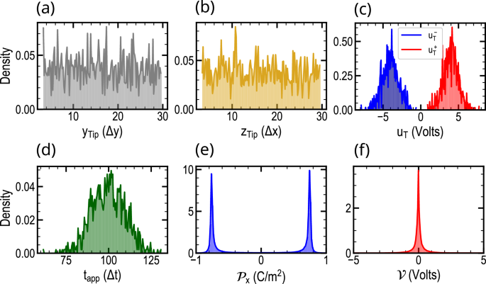
Each trajectory consisted of 10 distinct switching events, each programmed to last 200Δt, where Δt denotes the time-step employed in the phase-field simulations. Consequently, the total simulation duration spanned 2000Δt. For each event, the tip location (y_tip, z_tip) was randomly chosen on the sample surface, as depicted in Fig. 1a, b. The prescribed voltage u_T was randomly selected from the distribution shown in Fig. 1c. This distribution encompassed a range of voltages leading to electric fields approaching and exceeding the film’s coercive field, thereby ensuring frequent occurrences of electrical switching. Notably, voltages corresponding to electric fields below the coercive field, incapable of inducing domain reversal, were also included to train the model on the nuanced relationship between applied voltage and domain dynamics.

Fig. 1: Distribution of the training data and parameters in the training dataset.

a and b tip locations (y_tip−z_tip), c prescribed voltage of the AFM tip (u_T), d tip application time (t_app), e ferroelectric polarization (${{\mathcal{P}}}_{x}$), and f electrostatic potential (${\mathcal{V}}$) distributions.

Additionally, within each switching event spanning 200Δt, the tip application time t_app is randomly selected from the distribution shown in Fig. 1d. This distribution covers a range of approximately 50Δt–150Δt, representing diverse tip interaction durations. Throughout the remaining timesteps of each event, the domain undergoes relaxation without any applied voltage. This methodology ensures the model learns not only the temporal aspects of electrical switching but also the subsequent domain dynamics, including potential outcomes such as domain nucleation on the black electrode or back-switching to the initial state.

The microstructure state was then recorded at uniformly spaced time intervals of 20Δt, resulting in trajectories comprising 100 frames per simulation ({t₀, …, t₁₀₀}). Here, we conducted 1400 phase-field simulations to model ferroelectric domain switching on a system size of N_x × N_y × N_z = 16 × 32 × 32, producing $[{{\mathcal{P}}}_{x}^{{t}_{k}},{{\mathcal{V}}}^{{t}_{k}}]$ sequences with a shape of (100, 16, 32, 32, 2). The tip-related electrical boundary conditions [y_tip, z_tip, u_T] were recorded at the same intervals along the trajectory as scalar values, resulting in a tensor of shape (100, 3). The dataset was subsequently divided into a training dataset (1000 simulations), a validation dataset (200 simulations), and a test dataset (200 simulations).

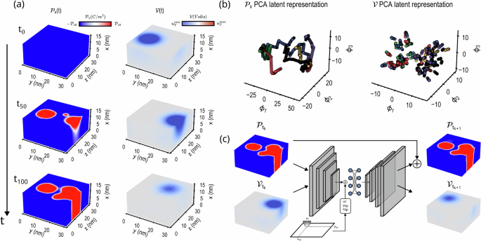
Figure 1e, f illustrates the distributions of polarization ${{\mathcal{P}}}_{x}$ and electrostatic potential ${\mathcal{V}}$ within the training dataset. An overview of a typical electrical domain switching trajectory from the training dataset is presented in Fig. 2a, depicting the evolution of the polarization and electrostatic potential variables, through a sequence of 10 tip-induced switching events.

Fig. 2: Illustration of the machine learning framework in the case of c⁺/c⁻ domains.

a Evolution of the polarization ${{\mathcal{P}}}_{x}$ and electrostatic potential ${\mathcal{V}}$ fields throughout a trajectory comprising 10 tip-induced switching events. b Visualization of selected trajectory examples for the ${{\mathcal{P}}}_{x}$ and ${\mathcal{V}}$ variables in the PCA lower-dimensional space. c The surrogate model takes the microstructure (${[{{\mathcal{P}}}_{x},{\mathcal{V}}]}^{{t}_{k}}$) and tip-related boundary conditions (prescribed voltage u_T and tip locations [y_tip, z_tip]) at time t_k as input to predict the next microstructural state at t_k+1.

The inherently complex nature of phase-field simulations generates highly intricate and nonlinear trajectories. In this study, we employed principal component analysis (PCA) to facilitate a clear and concise visualization of the switching trajectories^18,19 (Details on PCA are given in Supplementary Note 2). Figure 2b illustrates five arbitrarily chosen training dataset trajectories in the low-dimensional space delineated by the initial three principal components, for the polarization and electrostratic potential. In this representation, each switching event within a trajectory is characterized by abrupt directional changes, facilitating the observation of alterations in the boundary conditions across the simulation. Furthermore, this visualization approach effectively underscores the extensive diversity of scenarios encompassed within the generated datasets. Finally, the surrogate model architecture specifically tailored for the prediction of electrical switching in c⁺/c⁻ domains is presented in Fig. 2c.

The model was trained on the 1200 structures comprising the training/validation dataset over 100 epochs (refer to the “Methods” section for Training details). The training history, illustrated in Supplementary Fig. 1, depicts the evolution of the total ${{\mathcal{L}}}_{2}$ loss, as well as its two components (${{\mathcal{L}}}_{2}^{{{\mathcal{P}}}_{x}}$ and ${{\mathcal{L}}}_{2}^{{\mathcal{V}}}$), during the training process. Following training, the model’s performance was evaluated on the 200 test simulations, assessing the model’s ability to accurately forecast the microstructure using both direct one-step and long-timestep rollout strategies.

Evaluation of one-step prediction

The performance of one-step predictions is quantified using the ${{\mathcal{L}}}_{2}$ mean squared error (MSE) and ${{\mathcal{L}}}_{1}$ mean absolute error (MAE) metrics in Table 1 for the two output fields. Detailed metric computation procedures are described in the “Methods” section.

Table 1 Performance evaluation of the model for one-step prediction

The model demonstrates remarkable accuracy in forecasting subsequent microstructural states during electrical switching, achieving a quantitative MAE of 2.86 × 10⁻³ C/m² for the polarization field and 0.11 mV for the electrostatic potential. MSE values are also notably low, at 1.10 × 10⁻⁵ and 7.79 × 10⁻⁵ for ${{\mathcal{P}}}_{x}$ and ${\mathcal{V}}$, respectively, highlighting the model’s ability to capture the influence of boundary condition modifications and anticipate domain state dynamics.

While a model demonstrates accuracy for one-step predictions, it may not necessarily effectively replace high-fidelity methods, especially for longer time frames requiring full simulation unfolding. This can lead to a consistent accumulation of errors over the trajectories, highlighting the crucial need for robust models. Therefore, a thorough assessment is essential to evaluate the model’s ability to sustain error accumulation and ensure stable predictions over long time intervals.

Evaluation of unrolled prediction

For the rollout trajectories, simulations were initiated from diverse initial frames to evaluate the model’s robustness in scenarios with potential error accumulation. Our primary objective is to develop a surrogate that can effectively replace the high-fidelity phase field for a maximized number of frames while forecasting the switching process, leading to significant computational acceleration. As such, the model’s performance was analyzed across a spectrum of initial frames ranging from time t₀ to t₈₀ with the goal of predicting the complete morphological evolutionary pathway up to time t₁₀₀. Therefore, the surrogate unfolds the simulation from 20 (starting from t₈₀) to 100 (starting from t₂₀) timesteps.

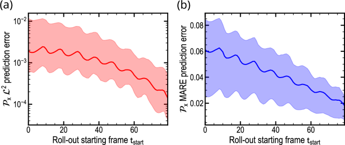
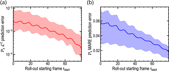
For each starting frame in the test dataset, the mean, 25th, and 75th quartiles of the MSE and the macro average relative error (MARE) were calculated over the 200 unrolled test trajectories for the ${{\mathcal{P}}}_{x}$ ferroelectric morphology (Fig. 3). The results highlight that simulations initiated at earlier frames tend to show higher prediction errors. In fact, data-driven surrogates naturally accumulate errors over long-time step inferences, as each prediction builds upon the previous one²⁶.

Fig. 3: Evaluation in unrolled prediction scenarios in the case of c⁺/c^- tip-induced domain switching.

a Evolution of the ${{\mathcal{L}}}_{2}$ error and b MARE during the unrolled trajectory. For each starting frame, complete domain switching trajectories are performed until the final frame at time t₁₀₀. Results are averaged over 200 test dataset simulations, with the solid line indicating the mean and the shaded region representing the interquartile range between the 25th and 75th percentiles.

Despite the observed sensitivity to initial conditions, the model displayed noteworthy robustness and stability. Even when starting from early frames and predicting all 10 switching events, no significant error accumulation was observed. The MARE stayed consistently below 10% across test samples, even for full simulation unrolling. In particular, the mean MARE hovered around 6% when starting from the t₀ state. Even better accuracy was achieved for predictions starting from slightly later frames, between t₂₀ and t₃₀ (corresponding roughly to 7 switching events). In these cases, the MARE dropped below 5%. Further reduction of the forecasted timesteps significantly enhances accuracy, ultimately yielding a 2% MARE.

Following these guidelines, it becomes feasible to define an error threshold for the surrogate, aligning with the accuracy requirements imposed by the application. This threshold would determine the acceptable number of predictable timesteps by the surrogate. Additionally, a hybrid solver approach could be envisaged, periodically incorporating high-fidelity phase-field iterations to restore microstructure state accuracy. This restored state could then be used for a new surrogate prediction sequence, as demonstrated in comparable literature²⁶.

Interestingly, both the mean and quartile error curves demonstrate consistent oscillations that coincide with individual switching events. This suggests that the model’s performance is sensitive to the specific initial state within a switching event. Notably, the error increases as the initial state approaches the end of a tip application period. This finding implies that the model performs best when starting its prediction at the very beginning of the tip application.

Illustration of forecasted trajectories

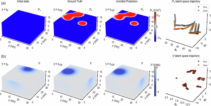
Figure 4 depicts the model’s ability to predict domain switching in a complete test simulation, covering the trajectory from t₀ to t₁₀₀ and including 10 switching events. The final outputs of ${{\mathcal{P}}}_{x}$ (Fig. 4a) and ${\mathcal{V}}$ (Fig. 4b) at t₁₀₀ closely match ground truth values. With high accuracy with minimal error accumulation during microstructure evolution, the surrogate proves its efficacy in anticipating domain dynamics during tip-induced electrical switching events. To provide a concise representation of the entire trajectory, both the ground truth and model predictions are depicted in the PCA space in Fig. 4 at each discrete timestep (t₀, …, t₁₀₀). Crucially, the dynamics of the reference solver are faithfully reproduced, capturing the overarching trends in the ${{\mathcal{P}}}_{x}$ and ${\mathcal{V}}$ sequences, respectively. Additional insights into the internal structure of the surrogate predictions are given from the 2D cross-sectional views presented in Supplementary Fig. 2.

Fig. 4: Illustration of an unrolled model prediction versus the high-fidelity reference solution, initialized at time t₀ for a test trajectory.

The microstructural states of a polarization (${{\mathcal{P}}}_{x}$) and b electrostatic potential (${\mathcal{V}}$) are depicted at the initial (t₀) and final (t₁₀₀) times. The prediction and high-fidelity trajectories for both variables are visualized in the low-dimensional space, utilizing the first three principal components.

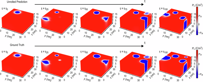
A detailed overview of the domain state evolution during switching forecasting is presented in Fig. 5. Here, the model serves as a complete replacement for the reference phase-field, unfolding a test simulation from t₀ to t₁₀₀. The corresponding domain state evolution is depicted at various time steps across the simulation (t₅, t₂₅, t₅₀, t₇₅, and t₁₀₀) for both the prediction and ground truth. Remarkably, the model closely mimics the true domain dynamics with impressive consistency throughout the simulation. While the model closely tracks the overall domain evolution, minor timing-related discrepancies exist. These mainly appear as slight overestimation of domain shrinkage (e.g., at t₂₅), ultimately having minimal impact on the final state. Conversely, the model occasionally diverges more significantly towards the trajectory’s end, missing a small domain formation (e.g., at t₂₅).

Fig. 5: Detailed temporal representation of the surrogate prediction for a c⁺/c⁻ tip-induced domain switching test trajectory.

Illustration of an unrolled model prediction versus the high-fidelity reference solution initialized at time t₀ for a test trajectory. Both microstructural states are represented at timesteps t₅, t₂₅, t₅₀, t₇₅ and t₁₀₀.

These findings highlight the model’s overall effectiveness in capturing domain dynamics but also point to areas for further improvement. By successfully replicating entire tip-induced switching sequences with a relative error below 10%, the model demonstrates a remarkable ability to capture the fundamental physical trend governing electrical domain switching. This achievement underscores the model’s potential to serve as a viable alternative to computationally demanding direct numerical solvers, offering a valuable compromise between computational efficiency and accuracy.

Unveiling generalization with unseen domain structure

While the model succeeds at predicting domain switching starting from single-domain states, a critical step for practical use involves its ability to handle unfamiliar initial domain structures. While pooling prior to electrical domain design might be an option in some cases, real-world applications may require operation on randomly configured domains. Therefore, a key question is whether the model can generalize its predictions to arbitrary conditions.

To assess the model’s ability to handle unseen domains, a new test set of 200 simulations (each with 10 switching events) was created. Here, these simulations did not start from single-domain states. Instead, they began with arbitrary domain structures resulting from natural domain formation. For each simulation, prior to tip-induced switching, the polarization was randomly initialized at each grid point, following a uniform distribution between ${{\mathcal{P}}}_{c0}$ and $-{{\mathcal{P}}}_{c0}$. Then, a classical domain formation process was simulated until equilibrium was reached (see the “Methods” section). The final domain state then became the starting point (t₀) for the tip-induced electrical trajectory. Supplementary Fig. 3 showcases representative switching trajectories initiated from diverse, realistic domain configurations. These complex starting states reflect real-world scenarios and lead to more intricate dynamics during tip applications, as seen in the figure.

The model’s performance on unseen initial states was directly assessed for unrolled trajectories. The results, reported in Fig. 6, demonstrate accuracy levels comparable to the single-domain cases, with consistently low MARE even for long-term predictions (100 frames), averaging below 6%. These findings highlight the model’s ability to generalize to unseen domain structures, accurately predicting 10 switching events without compromising accuracy.

Fig. 6: Evaluation in unrolled prediction scenarios for c⁺/c⁻ domain switching initiated from realistic domain state configurations.

a Evolution of the ${{\mathcal{L}}}_{2}$ error and b MARE during the unrolled prediction. For each starting frame, complete domain switching trajectories are performed until the final time t₁₀₀. Results are averaged over 200 test dataset simulations, with the solid line indicating the mean and the shaded region representing the interquartile range.

Finally, Fig. 7 illustrates the model’s predictions initiated from arbitrary domain configurations throughout an entire simulation. The ${{\mathcal{P}}}_{x}$ microstructure inferred by the surrogate is compared with the corresponding ground truth for the final states, along with its representation in the PCA space. Remarkably, even when starting from unseen initial configurations, the dynamical pathways produced by the surrogate exhibit significant agreement with the high-fidelity trajectories. These observations underscore the surrogate’s comprehension of the underlying evolution equation governing domain switching dynamics, thereby exhibiting remarkable generalization to unseen scenarios and enabling exploration of real-world applications.

Fig. 7: Illustration of an unrolled model prediction versus the high-fidelity solution, initialized at time t₀ from a realistic domain state configuration.

The polarization (${{\mathcal{P}}}_{x}$) microstructures are depicted at the initial (t₀) and final (t₁₀₀) times. The prediction and high-fidelity trajectories for both variables are visualized in the low-dimensional space, utilizing the first three principal components.

Electrical switching prediction of a/c domains

In this section, we address the case of electrical switching in a/c ferroelectric domain states, which are commonly examined in the field of domain and DW control engineering^46,47,48. These structures are characterized by mechanical boundary conditions that allow for both in-plane and out-of-plane polarization orientations. When subjected to a tip-induced electric field, such systems have the potential to exhibit both out-of-plane and in-plane domain switching. Thus, all components of the polarization vector (${{\mathcal{P}}}_{x}$, ${{\mathcal{P}}}_{y}$, ${{\mathcal{P}}}_{z}$) were taken into account during the training of the machine learning surrogate specifically developed for predicting a/c domain switching dynamics in this section.

Dataset

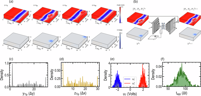
In the context of a/c domains, and more broadly, in analogous ferroelectric domain configurations featuring non-180° DWs, most research efforts have primarily focused on achieving precise control over the DWs displacement using tip scanning technique^{41,46,47,48,49,50}. In consideration of this, we tailored the dataset generation and model training process with the specific aim of developing a surrogate capable of precisely manipulating 90^∘ DWs through electrical tip scanning as illustrated in Fig. 8a.

Fig. 8: Illustration of the machine learning framework and training dataset in the case of a/c domains.

a Example depicting the evolution of the a/c domain structure and electrostatic potential throughout a training trajectory. Domain states are depicted at time t₀, t₂₀, t₄₁, and the final time t₆₂, highlighting various voltage applications during tip scanning trajectory. b Illustration demonstrating the surrogate model operations over the ${{\mathcal{P}}}_{x}$, ${{\mathcal{P}}}_{y}$, and ${{\mathcal{P}}}_{z}$ polarization components, along with the ${\mathcal{V}}$ electrostatic potential, specifically in the scenario of a/c ferroelectric domain switching. Distribution in the training dataset of c and d tip locations (y_tip−z_tip), e prescribed voltages of the AFM tip (u_T), and f tip application times (t_app).

To do this, a dataset comprising 1400 phase-field simulations was generated on a grid size of N_x × N_y × N_z = 8 × 32 × 32, with the microstructural state $[{{\mathcal{P}}}_{x},{{\mathcal{P}}}_{y},{{\mathcal{P}}}_{z},{\mathcal{V}}]$ stored at intervals of 20Δt. An illustration of the surrogate operation in the context of the a/c structure is provided in Fig. 8b, emphasizing the consideration and prediction of both the in-plane and out-of-plane polarization components. Adaptations made to the network architecture to accommodate this scenario are detailed in Supplementary Note 1.

Each trajectory began with the domain structure initialized with an in-plane a domain surrounded by out-of-plane c domains (Fig. 8a). This initialization was achieved through phase-field of a/c domain formation (see the “Methods” section), progressing from a random initial polarization noise to attain domain equilibrium before the commencement of the switching trajectory. It is worth noting that the location and orientation of the in-plane domain differed across various initial states within the dataset.

Subsequently, a random voltage was selected, and tip-induced switching was conducted by scanning the tip along with the 90° DW, emulating real-life tip scanning experiments. The decision to apply the tip on either the left or right side of the a/c domain was made randomly, resulting in occurrences of DW motion in both directions. The number of tip applications along the domain wall (DW) was randomly selected from a uniform distribution ranging between 3 and 8 applications. The tip locations (y_tip, z_tip) along a trajectory were determined based on the number of application steps, ensuring the tip scanned the entire film width along the DW (Fig. 8c, d). This approach aimed to cover a representative range of DW-tip interactions and DW motions. The prescribed voltage u_T was randomly selected from the distribution shown in Fig. 8e, encompassing both sub and low-coercive electric fields. This voltage selection ensured potential in-plane electric domain switching, enabling the surrogate to generalize across a broad spectrum of domain dynamics. Similarly to the previous case, each switching event lasted 200Δt, with tip application times randomly ranging from 50Δt to 150Δt, and the remaining timesteps were utilized for domain relaxation (Fig. 8f). Subsequently, the structure underwent relaxation for an additional 100Δt after the completion of tip scanning. A typical a/c domain switching training trajectory following this methodology is illustrated in Fig. 8a. Finally, the dataset was divided according to a 1000:200:200 training/validation/test ratio.

Evaluation of unrolled prediction

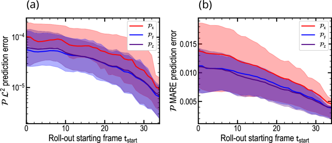
Following model training, we directly evaluated the surrogate in the scenario of unrolled a/c tip scanning domain switching prediction on the test dataset. The model was provided with an initial frame close to the start of the simulation (t₀–t₃₀) and was assessed by unrolling the entire simulation until the conclusion of tip scanning and final domain state relaxation. The ${{\mathcal{L}}}_{2}$ and MARE prediction errors for the in-plane and out-of-plane polarization components depending on the initial frame are reported in Fig. 9.

Fig. 9: Evaluation in unrolled prediction scenarios for a/c tip-induced domain switching.

a Evolution of the ${{\mathcal{L}}}_{2}$ error and b MARE during the unrolled prediction for the ${{\mathcal{P}}}_{x}$, ${{\mathcal{P}}}_{y}$ and ${{\mathcal{P}}}_{z}$ polarization components. For each starting frame, complete domain switching trajectories are performed until the final frame. Results are averaged over 200 test dataset simulations, with the solid line indicating the mean and the shaded region representing the interquartile range.

Our analysis reveals that the surrogate accurately predicts the domain state for all components, exhibiting a relative error below 2%, even when starting from the simulation onset. This underscores the surrogate’s capability to faithfully forecast the domain state throughout the entirety of a tip-scanning trajectory. Notably, errors in the out-of-plane polarization (${{\mathcal{P}}}_{x}$) are marginally higher than those observed in the in-plane counterparts, likely attributable to the prevalence of out-of-plane domains in a/c ferroelectric structures.

Interestingly, the overall errors are slightly lower than in the previous case of c⁺/c⁻ domains. This disparity can be attributed to the fact that the typical switching trajectory induced by tip scanning in the case of 90° DW control yields less variation in the global domain state relative to the multiple nucleation events of c⁺/c⁻ domains arising from the tip trajectory in the preceding section.

Illustration of forecasted trajectories

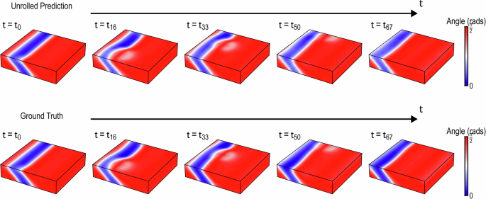
Figure 10 presents an illustration of the model performance over an entire tip-scanning trajectory using a simulation from the test dataset. In this simulation, the tip was biased with a voltage of −1.93 V and scanned along the DW by applying the voltage over five application steps. Figure 10 demonstrates the evolution of the a/c domain structure throughout the simulation, from the initial scanning to relaxation completion at the final time, t₆₇. It can be observed that the surrogate model adeptly reproduces the domain dynamics during the entire tip-scanning process, progressively moving the domain wall through tip-induced in-plane ferroelectric switching. Additional examples of switching trajectory predictions from test simulations are provided in Supplementary Figs. 4–6. Notably, the surrogate model accurately forecasts not only the final position of the domain wall after scanning but also the underlying domain state transitions. Hence, the proposed framework proves to operate as an effective alternative to traditional phase-field modeling for the entire trajectory length in applications related to 90° DW motion and control.

Fig. 10: Illustration of an unrolled model prediction versus the high-fidelity reference solution in the case of a/c domain switching under a tip bias of −1.93 V, initialized at time t₀ for a test trajectory.

Both predicted and ground truth microstructural states are represented at timesteps t₀, t₁₆, t₃₃, t₅₀ and at the final time t₆₇.

Computation efficiency

In this section, we analyze the acceleration provided by the machine learning surrogate model when compared to traditional approaches. The primary advantage of using a neural network surrogate lies in its significantly cheaper computational cost during inference, as opposed to direct numerical solvers. However, quantifying the speed-up achieved by a surrogate model presents a nuanced challenge due to hidden computational costs, such as dataset generation and model training.

To navigate this complexity, we initiate our analysis by focusing on the inference times of both approaches. Assuming the surrogate entirely substitutes the direct solver from time t₀, we report acceleration factors computed over the 200 test simulations in the case of unrolled simulations Table 2. This evaluation was conducted on both CPU and GPU material, enabling a fair comparison with simulations using traditional solvers. The analysis reveals significant performance gains with the surrogate, achieving speed-ups of 1390 on CPU and 2550 on GPU, confirming the surrogate’s potential to unlock demanding phase-field problems.

Table 2 Computational efficiency of the machine learning framework for domain switching forecasting

While our approach yields rapid inferences, acknowledging the initial computational investment in surrogate creation is crucial. We present dataset generation and model training times in Table 2 for a comprehensive cost overview. It is essential to emphasize that these results are contingent upon our specific computational material and methodology. Alternative computational configurations or numerical approaches for the phase field, such as employing finite-element methods instead of spectral methods to solve the PDEs set, may yield divergent execution times.

Discussion

This study presents a machine-learning surrogate for tip-induced electrical switching. Handling time-evolving electrical boundary conditions, the surrogate faithfully predicts polarization and electrostatic potential evolution across multiple switching scenarios. Its versatility spans diverse voltage, tip location, and application times, enabling exploration of vast parameter spaces in realistic settings. Remarkably, it maintains relative errors below 10% even over long timesteps inference. This fast time-stepper offers a 2500× speedup in morphology inference, paving the way for real-time simulations.

Generating training data for data-driven surrogates incurs substantial upfront costs, primarily due to dataset creation. Data augmentation leveraging physically plausible transformations offers a potential solution to mitigate this bottleneck. Additionally, transfer learning across diverse material parameters and system scales expands framework applicability, requiring minimal additional training data. Importantly, surrogate development constitutes a one-time investment. Subsequent use incurs negligible computational expense, unlocking the ability to solve previously intractable optimization problems requiring massive iterations.

In this article, we addressed vertical c⁺/c⁻ and a/c domain structures, showcasing the surrogate model’s ability to manage complex domain states with both in-plane and out-of-plane polarization components. This framework could be expanded to handle additional domain structures in 3D ferroelectrics, such as the 71°, 109°, and 180° domain walls in BiFeO₃ ferroelectrics^49,50, or the domain states found in (110) oriented PZT thin films^40,51.

Despite incorporating electrical boundary conditions, further development is necessary to create a comprehensive surrogate model for ferroelectric phase-field. Building on the current approach, integrating mechanical conditions like tip location, load, and misfit strain could emulate tip-induced switching and explore domain states in realistic mechanical scenarios¹⁷. Furthermore, in real-life contexts, parameters related to the experimental setup typically require calibration for accurate modeling. Therefore, an extension of the presented framework to accommodate additional tip parameters can be envisaged. For example, while the current framework operates with a fixed tip radius, we present a potential extension that includes varying tip diameters in Supplementary Note 5. This example illustrates possible adaptations of the existing framework to effectively address the constraints of real-life experimental setups.

With this work, we aim to provide a promising approach for utilizing phase-field modeling in addressing costly inverse problems through RL^40,41. Our framework lays the foundation for an AI agent that designs domain structures via electrical phase-field simulations. The AI, tasked with achieving a target state, could explore diverse tip locations, voltages, and durations to learn an optimal switching strategy through repeated attempts. Leveraging our efficient surrogate instead of the full phase-field model enables significantly faster learning while accurately capturing switching dynamics. We envision this framework significantly helping the design and comprehension of domain structures in modern DW nanoelectronics.

In conclusion, we presented a machine learning approach to accurately replicate tip-induced electrical switching in 3D ferroelectric phase-field simulations. The surrogate demonstrates remarkable accuracy over extended timescales, providing an efficient alternative to computationally expensive high-fidelity methods. Its ability to rapidly simulate electrical switching trajectories with dynamic boundary conditions creates new opportunities for the electrical design of ferroelectric materials at an unprecedented pace.

Methods

Phase-field modeling

In the context of phase-field simulations, the dynamic evolution of ferroelectric polarization is described by the TDGL equation^11,12,14:

$$\frac{\partial {P}_{i}({\boldsymbol{r}},t)}{\partial t}=-L\frac{\delta \psi }{\delta {P}_{i}({\boldsymbol{r}},t)},\quad (i=1,2,3)$$

(8)

where P_i(r, t) is the spontaneous polarization, L is a kinetic coefficient, ψ is the total free energy and r = (x, y, z) denotes the spatial vector in 3D. The total free energy includes the bulk, gradient, electric, and elastic free energy density

$$\psi ={\int}_{V}({\psi }_{{\rm {bulk}}}+{\psi }_{{\rm {grad}}}+{\psi }_{{\rm {elec}}}+{\psi }_{{\rm {elas}}})\delta V$$

(9)

The polarization was updated at each time step following the explicit scheme:

$${P}_{i}({\boldsymbol{r}},t+\Delta t)={P}_{i}({\boldsymbol{r}},t)+\frac{\partial {P}_{i}({\boldsymbol{r}},t)}{\partial t}\Delta t$$

(10)

where Δt is the time step for integration.

The bulk energy is described by

$$\psi ({P}_{i})={\alpha }_{i}{P}_{i}^{2}+{\alpha }_{ij}{P}_{i}^{2}{P}_{j}^{2}+{\alpha }_{ijk}{P}_{i}^{2}{P}_{j}^{2}{P}_{k}^{2},$$

(11)

where α_i, α_ij, and α_ijk are the second-, fourth- and sixth-order PZT Landau coefficients, which are taken from the literature⁵², and ${\alpha }_{1}=\frac{T-{T}_{0}}{2\epsilon C}$ refers to the dielectric permittivity ϵ, the Curie temperature T₀ and the Curie constant C.

The energy caused by the DWs is described by the gradient energy, which in a cubic system is calculated by

$${\psi }_{{\rm {grad}}}(\nabla {P}_{i})=\frac{1}{2}{G}_{ijkl}\left(\frac{\partial {P}_{i}}{\partial {x}_{j}}\frac{\partial {P}_{k}}{\partial {x}_{l}}\right),$$

(12)

where G represents the gradient energy coefficient tensor.

The electric energy is given by

$${\psi }_{{\rm {elec}}}({P}_{i},{E}_{i})=-{P}_{i}{E}_{i}-\frac{1}{2}{\epsilon }_{0}{\epsilon }_{r}{E}_{i}{E}_{j},$$

(13)

where E_i = −∇_iV is the electric field obtained by solving the electrostatic equilibrium:

$$\Delta V=-\frac{\rho -\nabla \cdot {\boldsymbol{P}}}{{\epsilon }_{0}{\epsilon }_{r}}$$

(14)

Here, ρ represents the electric charge, and −∇⋅P denotes the depolarization charges induced by the polarization. Electrostatic equilibrium is solved using the fast Fourier transform method (details in refs. ^18,53), with periodic boundary conditions along the y and z in-plane directions.

Tip-induced switching was emulated by adjusting the electrostatic potential under the tip in the Dirichlet boundary conditions at the top electrode (x = x_top). Consistent with many phase-field studies, the surface electrostatic potential was approximated using a Lorentz-like distribution of the applied bias u_T^14,54:

$$V({x}_{{\rm {top}}},y,z)={u}_{{\rm {T}}}\frac{{\gamma }^{2}}{{\gamma }^{2}+{r}^{2}},\quad V(0,y,z)=0$$

(15)

where γ is the half-width of the tip. The distance from the tip center, r, is calculated as $r=\sqrt{{({y}_{{\rm{tip}}}-y)}^{2}+{({z}_{{\rm{tip}}}-z)}^{2}}$, accounting for the varying tip location r_tip = x_top, y_tip, z_tip) across switching trajectories.

In microstructure evolution without tip influence, we assume complete charge screening at both the bottom electrode and the top surface. This configuration is employed during relaxation phases post-switching and for the initial domain formation prior to tip application sequence in unforeseen domain structure scenarios. Hence, short-circuit electrostatic conditions were applied:

$$V({x}_{{\rm {top}}},y,z)=V(0,y,z)=0\,{\rm {V}}$$

(16)

The elastic energy density is described by

$${\psi }_{{\rm {elas}}}({P}_{i},{\epsilon }_{ij})=\frac{1}{2}{C}_{ijkl}({\epsilon }_{ij}({\boldsymbol{r}})-{\epsilon }_{ij}^{0}({\boldsymbol{r}}))({\epsilon }_{kl}({\boldsymbol{r}})-{\epsilon }_{kl}^{0}({\boldsymbol{r}}))$$

(17)

where C is the elastic stiffness tensor, ϵ is the total strain and ϵ⁰ is the electrostrictive strain caused by the polarization as

$${\epsilon }_{ij}^{0}({\boldsymbol{r}})={Q}_{ijkl}{P}_{k}({\boldsymbol{r}}){P}_{l}({\boldsymbol{r}})$$

(18)

where Q is the electrostrictive tensor. The total strain contains the homogeneous and heterogeneous strains:

$${\epsilon }_{ij}({\boldsymbol{r}})={\epsilon }_{ij}^{s}+\delta {\epsilon }_{ij}({\boldsymbol{r}})$$

(19)

which is linked to the mechanical displacement u_i by

$$\delta {\epsilon }_{ij}({\boldsymbol{r}})=\frac{1}{2}\left(\frac{\partial {u}_{i}({\boldsymbol{r}})}{\partial {x}_{j}}+\frac{\partial {u}_{j}({\boldsymbol{r}})}{\partial {x}_{i}}\right)$$

(20)

The mechanical equilibrium equation σ_ij,j = 0, solved for the displacements, is given by (using Einstein notation) :

$${C}_{ijkl}\frac{{\partial }^{2}{u}_{k}({\boldsymbol{r}})}{\partial {x}_{j}\partial {x}_{l}}={C}_{ijkl}\frac{\partial {\epsilon }_{kl}^{0}({\boldsymbol{r}})}{\partial {x}_{j}}$$

(21)

The simulations were conducted on a 3D grid of N_x × N_y × N_z points with uniform spacing Δx/l₀ = Δy/l₀ = Δz/l₀ = 1, where ${l}_{0}=\sqrt{{G}_{110}/{\alpha }_{0}}\approx 1\,{\rm{nm}}$ (${\alpha }_{0}=| {\alpha }_{1}{| }_{T = 2{5}\,^{\circ }{\rm {C}}}$¹¹). Gradient energy coefficients followed ref. ¹¹: G₁₁/G₁₁₀ = 0.6, G₁₂/G₁₁₀ = 0, G₄₄/G₁₁₀ = 0.3. The time step was Δt = 0.02t₀, where t₀ = 1/(α₀L₀). For the c⁺/c⁻ domain state scenario, the PZT films were constrained by a −1% in-plane mismatch, aligning with a typical setting in PZT simulations⁴³. For the case addressing a/c domain structures, no lattice mismatch was applied. The other PZT parameters utilize values established in literature^11,43,55. A listing of these parameters and the associated normalization procedure is provided in Supplementary Note 6.

Training details

To enhance the stability of rollout predictions, we implemented a progressive noise augmentation strategy on the input training features. Inspired by error accumulation in real-world data (refs. ^18,56), Gaussian noise was incrementally increased along simulation trajectories. Notably, the target labels remained noise-free. The noise magnitudes for polarization and electrostatic fields were set at σ_P = 10⁻³ and σ_V = 10⁻⁵, respectively, conforming to the methodology established in ref. ¹⁸.

The model parameters were optimized during training using the Adam optimizer with a batch size of 32. The initial learning rate was set at 10⁻³ and gradually reduced to 10⁻⁶, following an exponential decay over during 100 epochs.

Error metrics

Mean squared error (MSE)

The mean squared error loss function ${{\mathcal{L}}}_{2}$ can be computed over the ${\{({Y}_{i},{X}_{i})\}}_{i = 1}^{N}$ training samples as

$${{\mathcal{L}}}_{2}({Y}^{{t}_{k+1}},{\mathcal{S}}({X}^{{t}_{k}}))=\frac{1}{N}\mathop{\sum }\limits_{i=1}^{N}{({Y}_{i}^{{t}_{k+1}}-{\mathcal{S}}({X}_{i}^{{t}_{k}}))}^{2}$$

(22)

where ${Y}^{{t}_{k+1}}$ is the microstructure labels obtained by real phase-field simulations and ${\mathcal{S}}({X}^{t})$ are the model outputs.

To assess rollout simulations, the score is averaged across each trajectory, such as

$${{\mathcal{L}}}_{2}=\frac{1}{MN}\mathop{\sum }\limits_{m=1}^{M}\mathop{\sum }\limits_{n=1}^{N}{({Y}_{m}^{{t}_{n+1}}-{{\mathcal{S}}}_{m}({X}^{{t}_{n}}))}^{2}$$

(23)

where M denotes the number of trajectories in the validation dataset and N is the number of frames per simulation.

Macro average relative error (MARE)

The macro average relative error (MARE) can be computed in the context of rollout evaluations by

$${\rm{MARE}}=\frac{1}{M}\mathop{\sum }\limits_{m=1}^{M}\frac{\mathop{\sum }\nolimits_{n = 1}^{N}| {Y}_{m}^{{t}_{n+1}}-{{\mathcal{S}}}_{m}({X}^{{t}_{n}})| }{\mathop{\sum }\nolimits_{n = 1}^{N}| {Y}_{m}^{{t}_{n+1}}| }$$

(24)

Mean absolute error (MAE)

The mean absolute error (MAE) ${{\mathcal{L}}}_{1}$ can be determined by

$${\rm{MAE}}=\frac{1}{N}\mathop{\sum }\limits_{n=1}^{N}| {Y}_{m}^{{t}_{k+1}}-{{\mathcal{S}}}_{m}({X}^{{t}_{k}})|$$

(25)

Computational material

The machine learning framework utilized in this study was implemented using TensorFlow2. The training procedure and assessments of GPU computational efficiency were conducted on an NVIDIA GeForce RTX 3080 with 10 GB of RAM. Dataset generation using the direct numerical solver and assessments of CPU computational efficiency were performed using an INTEL i9 CPU clocked at 5.1 GHz.

References

Scott, J. F. & Paz de Araujo, C. A. Ferroelectric memories. Science 246, 1400–1405 (1989).
Crassous, A., Sluka, T., Tagantsev, A. K. & Setter, N. Polarization charge as a reconfigurable quasi-dopant in ferroelectric thin films. Nat. Nanotechnol. 10, 614–618 (2015).
Sharma, P. et al. Conformational domain wall switch. Adv. Funct. Mater. 29, 1807523 (2019).
McGilly, L. J., Yudin, P., Feigl, L., Tagantsev, A. K. & Setter, N. Controlling domain wall motion in ferroelectric thin films. Nat. Nanotechnol. 10, 145–150 (2015).
Setter, N. et al. Ferroelectric thin films: review of materials, properties, and applications. J. Appl. Phys. 100, 051606 (2006).
Gonzalez Casal, S. et al. Mechanical switching of ferroelectric domains in 33–200 nm-thick sol–gel-grown PbZr0.2Ti0.8O3 films assisted by nanocavities. Adv. Electron. Mater. 8, 1–9 (2022).
Guo, E. J., Roth, R., Das, S. & Dörr, K. Strain induced low mechanical switching force in ultrathin PbZr0.2Ti0.8O3 films. Appl. Phys. Lett. 105, 012903 (2014).
Sharma, P. et al. Nonvolatile ferroelectric domain wall memory. Sci. Adv. 3, e1700512 (2017).
Sharma, P., Moise, T. S., Colombo, L. & Seidel, J. Roadmap for ferroelectric domain wall nanoelectronics. Adv. Funct. Mater. 32, 2110263 (2022).
Wang, J. et al. Ferroelectric domain-wall logic units. Nat. Commun. 13, 3255 (2022).
Li, Y. L., Hu, S. Y., Liu, Z. K. & Chen, L. Q. Effect of substrate constraint on the stability and evolution of ferroelectric domain structures in thin films. Acta Mater. 50, 395–411 (2002).
Chen, L.-Q. Phase-field models for microstructure evolution. Annu. Rev. Mater. Res. 32, 113–140 (2002).
Zhao, Y. Understanding and design of metallic alloys guided by phase-field simulations. npj Comput. Mater. 9, 94 (2023).
Wang, J. J., Wang, B. & Chen, L. Q. Understanding, predicting, and designing ferroelectric domain structures and switching guided by the phase-field method. Annu. Rev. Mater. Res. 49, 127–152 (2019).
Bortis, A., Trassin, M., Fiebig, M. & Lottermoser, T. Manipulation of charged domain walls in geometric improper ferroelectric thin films: a phase-field study. Phys. Rev. Mater. 6, 064403 (2022).
Vasudevan, R. K. et al. Domain wall geometry controls conduction in ferroelectrics. Nano Lett. 12, 5524–5531 (2012).
Alhada-Lahbabi, K., Deleruyelle, D. & Gautier, B. Phase-field study of nanocavity-assisted mechanical switching in PbTiO3 thin films. Adv. Electron. Mater. 10, 2300744 (2023).
Alhada-Lahbabi, K., Deleruyelle, D. & Gautier, B. Machine learning surrogate model for acceleration of ferroelectric phase-field modeling. ACS Appl. Electron. Mater. 5, 3894–3907 (2023).
Montes de Oca Zapiain, D., Stewart, J. A. & Dingreville, R. Accelerating phase-field-based microstructure evolution predictions via surrogate models trained by machine learning methods. npj Comput. Mater. 7, 1–11 (2021).
Li, W., Bazant, M. Z. & Zhu, J. Phase-field DeepONet: physics-informed deep operator neural network for fast simulations of pattern formation governed by gradient flows of free-energy functionals. Comput. Methods Appl. Mech. Eng. 416, 116299 (2023).
Lu, L., Jin, P., Pang, G., Zhang, Z. & Karniadakis, G. E. Learning nonlinear operators via DeepONet based on the universal approximation theorem of operators. Nat. Mach. Intell. 3, 218–229 (2021).
Raissi, M., Perdikaris, P. & Karniadakis, G. E. Physics-informed neural networks: a deep learning framework for solving forward and inverse problems involving nonlinear partial differential equations. J. Comput. Phys. 378, 686–707 (2019).
Hemmasian, A. et al. Surrogate modeling of melt pool temperature field using deep learning. Addit. Manuf. Lett. 5, 100123 (2023).
Fetni, S. et al. Capabilities of auto-encoders and principal component analysis of the reduction of microstructural images; application on the acceleration of phase-field simulations. Comput. Mater. Sci. 216, 111820 (2023).
Choi, J. Y., Xue, T., Liao, S. & Cao, J. Accelerating phase-field simulation of three-dimensional microstructure evolution in laser powder bed fusion with composable machine learning predictions. Addit. Manuf. 79, 103938 (2024).
Oommen, V., Shukla, K., Desai, S., Dingreville, R. & Karniadakis, G. E. Rethinking materials simulations: blending direct numerical simulations with neural operators. npj Comput. Mater 10, 145 (2024).
Peivaste, I. et al. Machine-learning-based surrogate modeling of microstructure evolution using phase-field. Comput. Mater. Sci. 214, 111750 (2022).
Xue, T., Gan, Z., Liao, S. & Cao, J. Physics-embedded graph network for accelerating phase-field simulation of microstructure evolution in additive manufacturing. npj Comput. Mater. 8, 201 (2022).
Oommen, V., Shukla, K., Goswami, S., Dingreville, R. & Em Karniadakis, G. Learning two-phase microstructure evolution using neural operators and autoencoder architectures. npj Comput. Mater. 8, 190 (2022).
Yang, K. & Cao, Y. Self-supervised learning and prediction of microstructure evolution with convolutional recurrent neural networks. Patterns 2, 100243 (2021).
Wu, P., Iquebal, A. S. & Kumar, A. Emulating microstructural evolution during spinodal decomposition using a tensor decomposed convolutional and recurrent neural network. Comput. Mater. Sci. 224, 112187 (2023).
Kemeth, F. P. et al. Black and gray box learning of amplitude equations: application to phase field systems. Phys. Rev. E 107, 025305 (2023).
Alhada-Lahbabi, K., Deleruyelle, D. & Gautier, B. Ultrafast and accurate prediction of polycrystalline hafnium oxide phase-field ferroelectric hysteresis using graph neural networks. Nanoscale Adv. 6, 2350–2362 (2024).
Karniadakis, G. E. et al. Physics-informed machine learning. Nat. Rev. Phys. 3, 422–440 (2021).
Samaniego, E. et al. An energy approach to the solution of partial differential equations in computational mechanics via machine learning: Concepts, implementation and applications. Comput. Methods Appl. Mech. Eng. 362, 112790 (2020).
Teichert, G. H., Natarajan, A. R., Van der Ven, A. & Garikipati, K. Machine learning materials physics: integrable deep neural networks enable scale bridging by learning free energy functions. Comput. Methods Appl. Mech. Eng. 353, 201–216 (2019).
Goswami, S., Yin, M., Yu, Y. & Karniadakis, G. E. A physics-informed variational DeepONet for predicting crack path in quasi-brittle materials. Comput. Methods Appl. Mech. Eng. 391, 114587 (2022).
Yang, H. & Demkowicz, M. J. Reinforcement learning strategy for control of microstructure evolution in phase field models. Comput. Mater. Sci. 231, 112577 (2024).
Mianroodi, J. R., Siboni, N. H. & Raabe, D. Computational discovery of energy-efficient heat treatment for microstructure design using deep reinforcement learning. arXiv:abs/2209.11259 (2022).
Vasudevan, R. K., Orozco, E. & Kalinin, S. V. Discovering mechanisms for materials microstructure optimization via reinforcement learning of a generative model. Mach. Learn.: Sci. Technol. 3, 04LT03 (2022).
Smith, B. et al. Physics-informed models of domain wall dynamics as a route for autonomous domain wall design via reinforcement learning. Digit. Discov. 3, 456–466 (2024).
Ronneberger, O., Fischer, P. & Brox, T. U-net: convolutional networks for biomedical image segmentation. In Proc. 18th International Conference on Medical Image Computing and Computer-Assisted Intervention—MICCAI 2015, Part III, Munich, Germany, October 5–9, 2015 Vol. 18 234–241 (Springer, 2015).
Cao, Y., Morozovska, A. & Kalinin, S. V. Pressure-induced switching in ferroelectrics: phase-field modeling, electrochemistry, flexoelectric effect, and bulk vacancy dynamics. Phys. Rev. B 96, 184109 (2017).
Wang, Y.-J., Li, J., Zhu, Y.-L. & Ma, X.-L. Phase-field modeling and electronic structural analysis of flexoelectric effect at 180° domain walls in ferroelectric PbTiO3. J. Appl. Phys. 122, 224101 (2017).
Cao, Y. & Kalinin, S. V. Phase-field modeling of chemical control of polarization stability and switching dynamics in ferroelectric thin films. Phys. Rev. B 94, 235444 (2016).
Khan, A. I., Marti, X., Serrao, C., Ramesh, R. & Salahuddin, S. Voltage-controlled ferroelastic switching in Pb(Zr0.2Ti0.8)O3 thin films. Nano Lett. 15, 2229–2234 (2015).
Nagarajan, V. et al. Dynamics of ferroelastic domains in ferroelectric thin films. Nat. Mater. 2, 43–47 (2003).
Gao, P. et al. Atomic-scale mechanisms of ferroelastic domain-wall-mediated ferroelectric switching. Nat. Commun. 4, 2791 (2013).
Wu, M. et al. Complete selective switching of ferroelastic domain stripes in multiferroic thin films by tip scanning. Adv. Electron. Mater. 10, 2300640 (2024).
Wu, M. et al. Facile control of ferroelastic domain patterns in multiferroic thin films by a scanning tip bias. ACS Appl. Mater. Interfaces 15, 11983 (2023).
Liu, D., Wang, J., Wang, J.-S. & Huang, H.-B. Phase field simulation of misfit strain manipulating domain structure and ferroelectric properties in PbZr(1–x)TixO3 thin films. Acta Phys. Sin. 69, 127801 (2020).
Hu, H.-L. & Chen, L.-Q. Three-dimensional computer simulation of ferroelectric domain formation. J. Am. Ceram. Soc. 81, 492–500 (1998).
Wang, J. J., Ma, X. Q., Li, Q., Britson, J. & Chen, L. Q. Phase transitions and domain structures of ferroelectric nanoparticles: phase field model incorporating strong elastic and dielectric inhomogeneity. Acta Mater. 61, 7591–7603 (2013).
Cao, Y., Li, Q., Chen, L.-Q. & Kalinin, S. V. Coupling of electrical and mechanical switching in nanoscale ferroelectrics. Appl. Phys. Lett. 107, 202905 (2015).
Wang, J., Shi, S. Q., Chen, L. Q., Li, Y. & Zhang, T. Y. Phase-field simulations of ferroelectric/ferroelastic polarization switching. Acta Mater. 52, 749–764 (2004).
Sanchez-Gonzalez, A. et al. Learning to simulate complex physics with graph networks. arXiv:abs/2002.09405 (2020).
Acknowledgements
This work has received the financial support of IPCEI France 2030 Programs POI and eFerroNVM together with ANR-23-CE24-0015-01 ECHOES project.
Author information
Authors and Affiliations
Contributions
K.A.L. got the original idea, ran the phase-field simulations, conceived the Machine Learning framework, performed the analysis, and wrote the manuscript. K.A.L., D.D., and B.G. worked on the development of the phase-field modeling code. All authors reviewed and discussed the manuscript.
Corresponding author
Ethics declarations
Competing interests
The authors declare no competing interests.
Additional information
Publisher’s note Springer Nature remains neutral with regard to jurisdictional claims in published maps and institutional affiliations.
Supplementary information
Rights and permissions
Open Access This article is licensed under a Creative Commons Attribution-NonCommercial-NoDerivatives 4.0 International License, which permits any non-commercial use, sharing, distribution and reproduction in any medium or format, as long as you give appropriate credit to the original author(s) and the source, provide a link to the Creative Commons licence, and indicate if you modified the licensed material. You do not have permission under this licence to share adapted material derived from this article or parts of it. The images or other third party material in this article are included in the article’s Creative Commons licence, unless indicated otherwise in a credit line to the material. If material is not included in the article’s Creative Commons licence and your intended use is not permitted by statutory regulation or exceeds the permitted use, you will need to obtain permission directly from the copyright holder. To view a copy of this licence, visit http://creativecommons.org/licenses/by-nc-nd/4.0/.
About this article
Cite this article
Alhada–Lahbabi, K., Deleruyelle, D. & Gautier, B. Machine learning surrogate for 3D phase-field modeling of ferroelectric tip-induced electrical switching. npj Comput Mater 10, 197 (2024). https://doi.org/10.1038/s41524-024-01375-7
Received:
Accepted:
Published:
Version of record:
DOI: https://doi.org/10.1038/s41524-024-01375-7