
Abstract
Material Testing 2.0 (MT2.0) is a paradigm that advocates for the use of rich, full-field data, such as from digital image correlation and infrared thermography, for material identification. By employing heterogeneous, multi-axial data in conjunction with sophisticated inverse calibration techniques such as finite element model updating and the virtual fields method, MT2.0 aims to reduce the number of specimens needed for material identification and to increase confidence in the calibration results. To support continued development, improvement, and validation of such inverse methods—specifically for rate-dependent, temperature-dependent, and anisotropic metal plasticity models—we provide here a thorough experimental data set for 304L stainless steel sheet metal. The data set includes full-field displacement, strain, and temperature data for seven unique specimen geometries tested at different strain rates and in different material orientations. Commensurate extensometer strain data from tensile dog bones is provided as well for comparison. We believe this complete data set will be a valuable contribution to the experimental and computational mechanics communities, supporting continued advances in material identification methods.
Background & Summary
Modeling material and component behavior using finite-element analysis (FEA) is critical for modern engineering. One key input into FEA is a material model, which describes the constitutive relationship between the loading conditions or history (such as applied deformation or force, deformation rate, temperature, etc.) and the resulting stress that develops in the material, in terms of a variety of material properties (such as Young’s modulus, Poisson’s ratio, yield stress, hardening parameters, etc.). The process of collecting experimental data is a key component of material characterization, and the process of identifying material model parameters is called model calibration; collectively, the entire process is often called material identification.
Historically, experimental data of material behavior has been limited to global measurements such as applied force and specimen extension. As a result, test specimens for model calibration typically had simple geometries such as tensile dog bones that are statically determined with homogeneous stress states. These simple experiments have the benefit of being relatively easy to perform, and trends in the data are often easy to identify manually. A main disadvantage, though, is that uniaxial stress states do not reflect real-world loading conditions. Nonetheless, models calibrated using simplistic, uniaxial data are routinely extrapolated and expected to predict material behavior under complex, multiaxial loading conditions. Additionally, to calibrate a complex material model, many experiments are required at different loading conditions (such as strain rates, temperatures, orientations, etc.), making model calibration time-consuming and expensive.
The development and maturity of full-field diagnostics, such as digital image correlation (DIC) and infrared (IR) thermography, have opened the door to more sophisticated methods of material model calibration. The availability of rich, full-field deformation data allows specimen geometries and applied forces or deformation to be complex, inducing heterogeneous stress states and a range of loading conditions (such as a range of strain rates and temperatures) in a single specimen. Thus, material models can be calibrated using data that more closely resembles the complex loading conditions a component of interest might experience during its lifetime. Additionally, by inducing a range of loading conditions in a single test, the number of tests required to calibrate complex material models may be reduced.
The move from simplified specimens like tensile dog bones to specimens of complex geometry for material identification has been recently christened “Material Testing 2.0” and has gained traction over the last few years1. There are many inverse techniques that capitalize on full-field deformation data for model calibration, such as the finite element model updating (FEMU) method, the constitutive equation gap method, the virtual fields method (VFM), the equilibrium gap method, and the reciprocity gap method; see Ref. 2 for a review of each of these methods. Efforts are widespread and on-going to improve these inverse techniques.
To support these code development and validation efforts—specifically for rate-dependent, temperature-dependent, and anisotropic metal plasticity and failure material models—we provide here a thorough experimental data set for 304L stainless steel sheet metal. Seven different unique specimen geometries were tested at two different deformation rates and in three different material orientations, with repeats of each configuration. Both full-field DIC displacement and strain data, as well as full-field IR temperature data, are provided for all specimens. Moreover, data is provided in both the raw format (i.e. tif images for DIC measurements and seq files for IR measurements), as well as a post-processed format where everything has been synchronized temporally and registered spatially. The raw data allows consumers the opportunity to tailor the processing workflow for their specific applications using software of their choice, while the post-processed data allows consumers to directly employ the data without the need to reprocess it. Additionally, extensometer strain data is provided for tensile dog bones tested at three strain rates and in three material orientations, facilitating comparisons between so-called traditional calibration approaches and emerging novel calibration methods. We believe this complete data set will be a valuable contribution to the experimental and computational mechanics communities, supporting continued advances in material identification methods.
Methods
Experimental Procedure
Specimen Fabrication
All test specimens were fabricated from a single rolled sheet of 304L stainless steel, nominally 1.5 mm thick. This material was selected because it is of particular interest for many applications at Sandia National Laboratories, while also widely used in industry. The sheet was cold rolled and then solution annealed and pickled. The complete metallurgical test report is provided in the data repository3 (see Section Data Records). Seven unique geometries, along with standard tensile dog bones, were tested. Schematic illustrations of the specimens are shown in Fig. 1, and complete drawings of the nominal dimensions are provided in the data repository3 (see Section Data Records). Specimens were fabricated in three orientations, along the rolling direction, transverse to the rolling direction, or at a 45° diagonal angle to the rolling direction of the sheet metal. More information on the specimen design for our original purposes is found in4,5,6.

Schematic illustrations of the seven unique geometries and tensile dog bone, with overall dimensions shown in millimeters. The horizontal dashed lines and blue rectangles represent the approximate location of the grips (i.e. the portion of the sample between the dashed lines is the region of interest). Complete drawings of the nominal dimensions are provided in the data repository3. The coordinate system origin is located at the bottom-left corner of each specimen, with the X axis horizontal and the Y axis vertical.
Mechanical Test Procedure
Specimens were tested on a dual-actuator, 77.8 kN (17.5 kip) capacity, custom load frame, shown in Fig. 2. The load frame was configured such that two actuators were placed inline horizontally, with each actuator moving at the same rate in opposing directions along the same axis, allowing the center of the specimens to approximately stay in the same location in the center of the field-of-view of the DIC and IR cameras. Each grip had anti-rotate bars that slid between two sets of guides, to stiffen the frame and reduce off-axis grip motion. The axial displacements of the hydraulic wedge grips were measured using linear variable differential transformers (LVDT, Model MHR-500, ±12.7 mm (0.500 in.) range) relative to a centrally located datum, as a means for more accurate grip displacement measurements.

Representative experimental setup for tensile testing of 304L sheet metal specimens of unique geometries and tensile dog bones, with DIC measurements on one side and IR measurements on the reverse. Here, an X-specimen is shown after failure.
The left hydraulic wedge grip (MTS Series 647) had a 111 kN (25 kip) load cell (Interface, Model 1220ACK-25K) inline with the left actuator (Miller, DH-67B4B). The right actuator and hydraulic wedge grip matched the left. For some tests, an additional 6-degree-of-freedom (6DOF) axial-torsion load cell (Interface, Model 6A175C-Q11) was mounted inline with the right actuator, providing forces and moments in all three directions. The capacities were 50 kN for the lateral loads, 100 kN for the axial load, and 5000 Nm for the moments.
Specimens of the seven unique geometries were tested to failure at a nominal grip velocity of either 2.5 ⋅ 10−3 mm/s/grip (5.0 ⋅ 10−3 mm/s total extension rate, labeled “slow”) or 2.5 mm/s/grip (5.0 mm/s total extension rate, labeled “fast”). For some specimens, a thermal load was additionally applied by locally heating the specimens with a radiative heat gun, in order to create a temperature rise that was independent of the mechanical deformation. The tensile dog bones were tested at the same fast and slow grip velocities, as well as an intermediate grip velocity of 8.0 ⋅ 10−2 mm/s/grip (1.6 ⋅ 10−1 mm/s total extension rate, labeled “medium”). These rates led to three nominal strain rates of approximately 1.0 ⋅ 10−4, 3.2 ⋅ 10−3, and 1.0 ⋅ 10−1 s-1 and times to failure of 1.9 hours, 160 seconds, and 5 seconds. The loading direction for all specimens was tensile along the Y axis of the specimen, following the coordinate system defined in Fig. 1. Note that in the actual test frame shown in Fig. 2, the Y axis was oriented horizontally.
DIC Measurements
For the tensile dog bones, which were tested first chronologically in the test series, several different patterning methods for DIC were evaluated on the different specimens. Due to the high strain-to-failure of 304L in conjunction with poor adhesion of paint to stainless steel, many of the patterns degraded and debonded in the localized necking region. However, only a virtual extensometer was extracted from the dog bones (as described in Section Tensile Dog Bones), utilizing only displacement data at the edges of the gauge section, where strains were lower and the DIC patterns remained intact. In the end, a suitable speckle pattern that maintained its integrity up to failure was obtained by spray painting white paint speckles onto the bare metal specimen with no solid base layer of paint underneath. Cross-polarized light was then used, which blocked specular reflections from the bare metal and allowed diffuse reflections from the white paint to pass to the camera, leading to a DIC pattern with a black background and white features7. This robust pattern was then used for all of the unique geometry specimens. Figure 3 shows a representative DIC pattern.

Representative DIC pattern for bespoke specimen O1-1, with a magnified inset showing a representative subset of size 23 × 23 px2.
Stereo DIC was performed using the hardware parameters specified in Table 1. For the majority of the tests, stereo DIC was performed on one side of the specimen with IR measurements on the other side, as shown in Fig. 2. For a few tests, two back-to-back stereo DIC systems were employed, with optical cameras viewing both sides of the specimen.
To perform a photogrammetry calibration of the stereo DIC systems, images of a standard dot-grid calibration target (Correlated Solutions) were collected at one or more times during each test day. The target was rotated, tilted, and translated throughout the entire calibration volume (i.e. the volume defined by the intersection of the field-of-view and depth-of-field of both cameras).
IR Measurements
For the majority of the tests, IR thermography measurements were made on the back side of the specimens using a FLIR A655sc long-wave (7.5–14 μm) IR camera operated at 50 Hz. (For a few tests, IR measurements were omitted when two back-to-back stereo DIC systems were employed instead.) The specimens were painted with a matte black paint (VHT brand, flat black), which maintained its integrity up to failure.
Post-Processing
Global Data
Global data (one-dimensional curves) included with this data set consist of the resultant force along the direction of loading from the standard uniaxial load cell, the total specimen extension as measured from the two LVDTs mounted to each grip, and the time. Additionally, for some specimens, the resultant forces and moments from the 6DOF load cell are also included. Figure 4 presents representative force-extension data.

Representative global data for bespoke specimen O1-1, including force from the standard load cell, forces and moments from the 6DOF load cell, and overall specimen extension as measured from the two LVDTs. (Time is also included in the global data, though not shown here).
Some data was collected before the test commenced. Therefore, the start of the test was defined by fitting a line to the force-vs-time data between 0.5–2 kN, and then extrapolating the line to a force of 0 kN. The time and extension were both zeroed based on this point. Global data was initially collected with a high frequency sampling rate through the MTS software, and then linearly interpolated and downsampled to match the DIC time vector.
DIC Data
Image Correlation and Strain Calculation
The stereo DIC systems were calibrated with a pinhole camera model and a third-order radial distortion model, using the images of dot-grid calibration target. For the tests with two back-to-back systems, each stereo system was calibrated independently, and the two DIC point clouds were registered to a common coordinate system as described below.
DIC images were analyzed according to the parameters specified in Table 2. Where possible, the region-of-interest (ROI) of the image was determined by binarizing the image based on a manually defined intensity threshold to separate the patterned specimen from the dark background. Where a single threshold was insufficient, the ROI of the image was drawn manually. After correlation, a best-plane fit was performed in the DIC software to set the Z axis perpendicular to the DIC point cloud of the nominally flat, undeformed specimen. Strains were then computed in the DIC software according to the parameters in Table 2. The data was exported for further analysis in MATLAB.
Spatial Registration
Each DIC data set was registered to a coordinate system based on the nominal specimen geometry (Fig. 1) as follows:
-
1.
The original location of the undeformed DIC point cloud as exported from the DIC software is shown in Fig. 5 (left). Rotations about the X and Y axes of either ±90o or 180o were determined manually and applied first in order to have the same approximate orientation for the DIC point cloud as the nominal specimen geometry.
Fig. 5 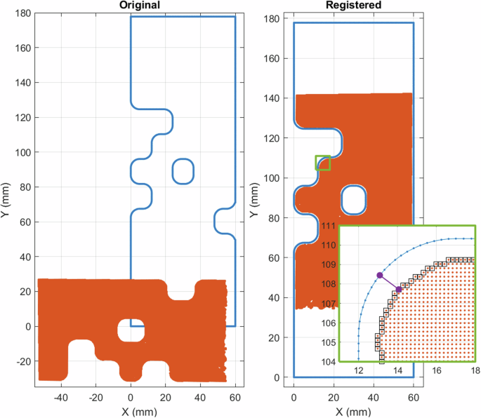
Example of the process used to spatially register the undeformed DIC point cloud (orange dots) to the nominal specimen geometry (blue outline), for bespoke specimen O1-1. (left) Original location of the DIC point cloud as exported from the DIC software. (right) Registered location of the DIC point cloud. (inset) Magnified view of the registered DIC point cloud, with the boundary nodes of the point cloud shown in black squares, and a representative distance between the DIC point cloud boundary node and the nominal specimen geometry boundary shown with the purple line.
-
2.
Initializations for the rotation about the Z axis and translations along the X and Y axes were determined manually and applied to approximately center the DIC point cloud within the nominal specimen geometry boundary.
-
3.
Translation along the Z axis was set to \(\pm \frac{T}{2}\) mm, where T = 1.50 mm is the nominal thickness of the specimen. This translation placed the undeformed point cloud on the appropriate surface of the specimen (either front or back).
-
4.
Nodes in the DIC point cloud that were on the boundary of the ROI or on the boundary of an interior hole were identified using the MATLAB function boundary; these boundary nodes are shown as black squares in the magnified inset of Fig. 5. Nodes that were along the top and bottom of the ROI (i.e. maximum and minimum Y-coordinate values of the DIC point cloud) were discarded, since the distance from these boundary points and the actual specimen edge was somewhat arbitrary based on the grip location, which was not precisely controlled.
-
5.
Because a local, subset-based DIC software was used, there was a gap between the boundaries of the the DIC point cloud and the actual edge of the specimen, equal to approximately half the subset size. The distance from each boundary node in the DIC point cloud to the closest node on the nominal geometry edge was computed; an example distance vector for a single boundary node is shown as the purple line in the magnified inset of Fig. 5.
-
6.
An optimization algorithm was used to identify the translations in X and Y directions and rotation about the Z axis that minimized the standard deviation of the distances between the DIC point cloud boundary nodes and the nominal geometry edge. Said another way, the optimization algorithm sought to make the gap between the edge of the DIC boundary nodes and the edge of the specimen constant. An example of a registered DIC point cloud is shown in Fig. 5 (right).
-
7.
A separate coordinate transformation was generated for each undeformed specimen. The coordinate transform was then applied to the deformed positions of the DIC point cloud at all time steps using the function pctransform in MATLAB.
-
8.
Displacements were recomputed based on the transformed positions of the deformed point cloud.
-
9.
The strains computed in VIC-3D were rotated to the new coordinate system according to:

where E* is the strain tensor rotated into the final coordinate system, E is the strain tensor computed in VIC-3D with the best-plane-fit VIC-3D coordinate system, and R is the rotation matrix arising from the registration process. Representative contour plots of the registered strains are presented in Fig. 6. (Note that the rotation matrix R is a 3 × 3 matrix and may involve rotations about all three axes. However, the strain tensor E is only 2 × 2, since only surface strains are available from optical DIC. Therefore, the Z components of the strain tensor were set to zero (i.e. Ezz = Exz = Eyz = 0) in Eqn. (1). This adaptation of the 2D strain tensor to a 3D matrix representation is only valid for rotations in increments of 90o about the X axis and Y axis.)

Representative strain data for bespoke specimen O1-1 after the spatial registration process was applied. Contours are shown at the time step of maximum force and are plotted in the reference configuration. Color bars represent strain in mm/mm; grey regions represent strains that are above/below the maximum/minimum color bar values.
IR Data
Temperature Calculation
Radiance was converted to temperature using ResearchIR software and the SDK for MATLAB8,9 and a FLIR factory camera calibration, with the settings shown in Table 3. Since emissivity of the paint was not explicitly measured, the emissivity is bounded by literature reference values10,11. Two temperature fields were computed, based on these bounds for the specimen emissivity.
Temporal Synchronization
The IR data was synchronized to the DIC time vector during post-processing as follows:
-
1.
The final failure of the specimen occurred abruptly within the time of a single image exposure. The frame in which specimen failure occurred was manually identified in both the DIC and the IR image sequences.
-
2.
The IR time vector was shifted to the DIC time vector based on this common point of failure.
-
3.
For each pixel in the IR image, the temperature data was linearly interpolated from the shifted IR time vector to the DIC time vector.
Spatial Registration
The IR data is inherently in an Eulerian (pixel-based or spatial) frame of reference while the DIC data is inherently in a Lagrangian (material-based) frame of reference. The IR data was therefore mapped to the DIC point cloud using a two-stage process that assumes the IR camera was perpendicular to the specimen.
First, the IR data of the undeformed specimen was registered to the coordinate system based on the nominal specimen geometry (Fig. 1) using the same procedure as for the DIC data (Section Spatial Registration, Steps 1–6). The one difference was in Step 4, where the boundary of the specimen and the holes in the IR image of the undeformed specimen were manually traced; these boundary nodes are shown as yellow squares in Fig. 7a. After registration, the average distance between the manually traced boundary nodes (yellow squares in Fig. 7b) and the nominal specimen geometry boundary (blue outline in Fig. 7b) was between 0.1–0.6 mm, indicating decent registration.

Example of the process used to spatially register the IR data (gray scale image) to the DIC point cloud (orange dots), for bespoke specimen O1-1. Note that the gray scale temperature range has been artificially adjusted for better visibility (a) Original IR image with the manually defined boundary nodes shown in yellow squares. (b) Registered IR image for the undeformed specimen, with the nominal specimen geometry (blue outline), registered DIC point cloud (orange dots), and registered IR boundary nodes (yellow squares) all overlaid. (c) Registered IR image for the deformed specimen at maximum force, with the deformed DIC point cloud overlaid.
Second, the IR data of the deforming specimen at each time step was mapped to the deformed DIC point cloud as follows:
-
1.
The coordinate transformation determined in the first stage for the undeformed IR image was applied to each IR image of the deforming specimen.
-
2.
The deformed coordinates of the DIC point cloud were overlaid onto the transformed IR image of the deformed specimen, as shown in Fig. 7b-c. Visually, the two data sets are well aligned, keeping in mind that there should be a gap of approximately one half the subset size between the edge of the DIC point cloud and the edge of the actual specimen shown in the IR image.
-
3.
The deformed IR data was linearly interpolated to the deformed DIC point cloud at each time step. A representative contour plot of the temperature field mapped to the DIC point cloud is presented in Fig. 8.
Fig. 8 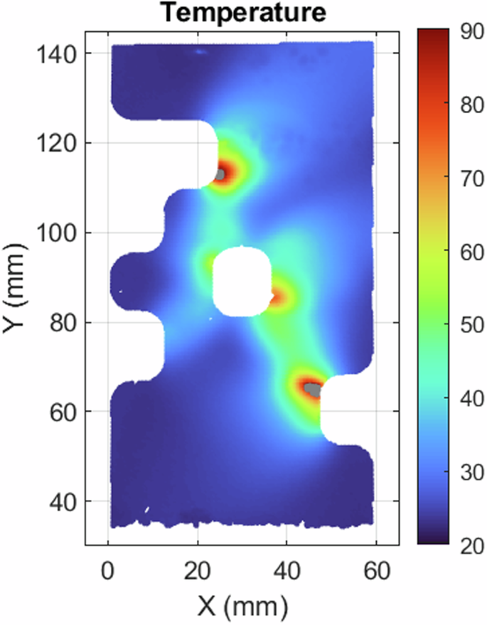
Representative temperature field for bespoke specimen O1-1 after mapping to the DIC point cloud. The contour is shown at the time step of maximum force and is plotted in the reference configuration. The color bar represents temperature in oC; grey regions represent temperatures that are above/below the maximum/minimum color bar values.

Tensile Dog Bones
Image Correlation and Coordinate System
DIC images were analyzed according to the parameters specified in Table 2. After correlation, a best-plane fit was performed in the DIC software to set the Z axis perpendicular to the DIC point cloud of the nominally flat, undeformed specimen. The Y axis was then manually oriented with the longitudinal axis of the undeformed specimen, and this coordinate transformation was applied to all time steps in the DIC software.
Virtual Extensometer
In contrast to the unique specimen geometries, the primary utility of the tensile dog bones is to generate a uniaxial state of stress in the uniform gauge section. Therefore, a virtual extensometer was extracted from the full-field DIC data along the longitudinal axis of the specimen. First, the location of maximum strain at the center of the necking region, in the image immediately prior to failure, was visually identified from the contour plot of the longitudinal strain field (point P0 in Fig. 9). Then points P1 and P2 were selected along the sample center line ±11 mm from P0 in the reference (undeformed) configuration. This virtual extensometer gauge length (L0 = 22 mm) was selected such that the end points would be outside of the localized necking region, yet remain in the field of view for all time steps of interest for all tests. The longitudinal displacements, V, were extracted for points P1 and P2, and the engineering strain along the longitudinal axis was computed as:

Representative tensile specimen, showing the location of P0 in the center of the necked region and the locations of P1 and P2 marking the edges of the virtual extensometer. The contour overlay represents the Hencky strain in mm/mm. Note that in this view, the Y axis is horizontal.
IR Data
Three of the transverse tensile dog bones additionally had IR data on the back side—AT4 (fast), BT4 (medium), and CT4 (slow). The measured radiance was converted to temperature and temporally synchronized to the DIC time vector using the same procedure as for the unique geometries (Section IR Data). However, the same spatial registration procedure could not be used because the field-of-view (FOV) of the DIC images was too small and did not have sufficient fiducials (i.e. the radiused portion of the dog bone was not visible) to allow the DIC data to be registered to the nominal geometry coordinate system. Therefore, a simplified registration process was developed as follows, to extract the temperature at the three points used in the virtual extensometer definition (Fig. 9):
-
1.
The location of the maximum temperature in the necking region, just prior to failure, was identified in the IR data. It was assumed that this point corresponded to point P0 of maximum strain identified from the DIC data on the other side of the specimen.
-
2.
The DIC displacement of point P0 was computed from the undeformed specimen to the time step just prior to failure.
-
3.
The DIC displacement was scaled from millimeters to pixels in the IR image using the IR image scale of 4.09 px/mm.
-
4.
The pixel in the undeformed IR image corresponding to point P0 was identified using the scaled displacement from the previous step.
-
5.
The pixels in the undeformed IR image corresponding to points P1 and P2 were selected at ±45 px from P0, which corresponds to ±11 mm when scaled by the IR image scale.
-
6.
The DIC displacements of points P0, P1, and P2, when scaled by the IR image scale, were used to track the material points through the series of IR images.
Features of the Material Behavior
While the primary focus of this data set is on full-field, heterogeneous DIC and IR data for Material Testing 2.0, one clear benefit of simple, uniaxial tests is the ability to probe a single variable at a time (e.g. strain rate, temperature, or material orientation) to gain intuition about the behavior of the material. Figure 10 presents representative data from the tensile dog bones. In the left subplot, mild anisotropic plasticity is clearly observed, with the rolling orientation having the highest plastic hardening, followed by the transverse orientation and the diagonal orientation. In the middle subplot, viscoplastic behavior (i.e. strain rate dependence) is clearly observed in the initial yield and hardening (strains less than 0.2 mm/mm). At higher strains, the slow tests appear to harden more than the medium and fast tests; however, this behavior is caused by significant temperature rise in the medium and fast tests, shown in the right subplot. The temperature rise is caused by the conversion of plastic work into heat and consequent material softening, which is accentuated at faster strain rates.

Representative tensile dog bone data showing (left) anisotropic plasticity, (middle) intertwined rate dependence and temperature dependence, and (right) temperature rise resulting from the conversion of plastic work into heat. The temperature was extracted from the center of the neck region (P0 in Fig. 9), and local Lagrange strain computed in the DIC software is reported instead of extensometer strain to emphasize the higher local strain in the neck region.
Data Records
Overview
The complete data records—as described in the following sections and illustrated notionally in Fig. 11—are stored in the Figshare+ repository3 and are freely available at https://doi.org/10.25452/figshare.plus.25483534. In the top level of the repository, there is a folder called MetaData (teal box in Fig. 11) that contains the complete specimen drawings, the complete test matrix of all specimens tested and the corresponding test conditions, and the metallurgical test report provided by the supplier for the lot of 304L sheet metal used here. Also in the top level of the repository, there is a zip folder called Movies (yellow box in Fig. 11), which contains a brief movie for every specimen, showing the displacements, strains, raw DIC image from one of the cameras, force-extension curve, and either thickness change (for specimens with two back-to-back stereo DIC systems) or IR temperature. These movies are included to give the consumer an idea of the specimen response before downloading the complete data set.

Notional illustration of the folder structure of the data repository.
Nominal Specimen Geometry
The data records are first organized by specimen geometry into four folders: D-Specimen, X-Specimen, BespokeSpecimens, and TensileDogBone (blue box in Fig. 11). Within each geometry folder, there is a file named *NominalGeometry.mat (green boxes in Fig. 11), which contains two variables: bOut is a matrix of the X − Y coordinates, in millimeters, of the outer boundary of the specimen; bHole is a cell array, where each cell contains a matrix of X − Y coordinates of the boundary of each hole in the specimen. Together, these matrices describe the X − Y coordinates of the boundaries of the nominal specimen geometries as specified by the specimen drawings in the repository. These are the coordinates that were used to spatially register the DIC and IR data to the nominal specimen geometry coordinate system as described in Section Post-Processing.
Post-Processed data
Within each specimen geometry folder (blue box in Fig. 11), the data records are grouped by test date (orange box in Fig. 11), with the folder names following the convention of YYMMDD, where Y stands for “year”, M stands for “month”, and D stands for “day”. Within each test date folder, there are folders with the specimen names tested that day (purple box in Fig. 11).
Within each specimen folder (purple box in Fig. 11), there is a *Data.mat file, which contains all of the post-processed data that has been spatially registered and temporally synchronized as described in Section Post-Processing. MAT-files are binary MATLAB files that store workspace variables; version 7.3 was used here to accommodate the large file size12. The specific variables are listed in Table 4. MAT-files saved with version 7.3 can also be read into Python using the PyPI function mat7313 or the h5py package14. (Note that the SciPy function loadmat only supports version 7.2 or lower and will not work for these version 7.3 MAT-files.) For specimens with two stereo DIC systems, the data is split into three files, with the global data (time, extension, and force) in the *Data.mat file, and the DIC data for each system in *Sys0-Data.mat and *Sys1-Data.mat files. In the *Data.mat files, some values may be NaN (i.e. “Not a Number”), where data is missing at a particular point in time and/or space.
Raw DIC and IR Files
Also within each specimen folder (purple box in Fig. 11), there is a zip folder called DIC-Images, which contains the original *.tif images of the deforming specimen acquired by the two DIC cameras of the stereo system. For specimens with two stereo DIC systems, the images are separated into two zip folders called DIC-Images-Sys0 and DIC-Images-Sys1. For the specimens with IR data, there is a zip folder called IR, which contains the original *.seq file acquired by the IR camera using the ResearchIR software. These *.seq files may be viewed and edited with either ResearchIR software or with the MATLAB SDK provided by FLIR8,9.
Within each test date folder (orange box in Fig. 11), there are also one or more zip folders that contain images of the DIC calibration target acquired on the date of the test (gray box in Fig. 11). The DIC calibration folder and the dot spacing of the target associated with each specimen are specified in the test matrix included in the MetaData folder in the repository (teal box in Fig. 11).
With these raw images, a consumer of this data set may reprocess the DIC images with different DIC software and user-defined settings. Additionally, a consumer may develop their own temporal synchronization and spatial registration post-processing algorithms to combine the DIC and IR data.
Tensile Dog Bones
The tensile dog bone data records are similarly organized into folders first by test date (orange box in Fig. 11) and then by specimen name (purple box in Fig. 11). Within each specimen folder, there is a *Data.mat file, which contains the global data associated with the tensile dog bone specimen, specifically the variables listed in Table 5.
Technical Validation
Global data
The LVDTs were verified at the time of use by a micrometer (Boeckler, Model 1398D, calibrated at the Primary Standards Laboratory at Sandia National Laboratories and traceable to the International System of Units (SI)) for better than 1% accuracy relative to current reading. The grip LVDT measurements had a standard deviation of approximately 0.5 μm (0.00002 in).
The standard load cell was calibrated onsite by MTS, traceable to the SI, for better than 1% accuracy relative to current reading. The standard load cell measurements have a standard deviation of approximately 2 N (0.5 lbf).
The 6DOF load cell was calibrated by the manufacturer at the time of purchase, a few months before it was employed for these tests. The accuracy of the 6DOF load cell measurements depends on the loading conditions. During calibration, when the applied load was 100 kN axially (maximum capacity), errors for all six DOFs were less than 0.02%; this condition most closely resembles the test conditions in this work, where the loading was predominately axial with small lateral forces and moments. When the applied load was 50 kN laterally (maximum capacity), errors were as high as 1.12%. When the applied load was a combination of either an axial or lateral force of 5 kN plus a moment of 5 kNm, errors were less than 0.31%.
Errors for the 6DOF load cell measurements reported here, however, may be larger than the manufacturer’s specifications, since effects of the specific signal conditioner and custom cables used here were not included in the manufacturer’s calibration. These effects could account for the discrepancies between the standard load cell and the 6DOF load cell axial force readings, which were typically 1% of applied load prior to failure. Because the standard load cell was calibrated onsite and included these equipment-specific effects, the force measurements from it are more trustworthy than those from the 6DOF load cell.
In the slow tests (specimens XR5, XT10, O1-3, O5-4, O14-3, O15-3, and O18-3), there are occasional drops in the force that are recovered with continued loading. These features are attributed to the anti-rotate bars mounted to the actuators momentarily catching on the guides and then releasing. They are not attributed to grip slip because (a) grip slip is expected to be worse for the faster tests, yet the features appear only on the slow tests, and (b) unloading and reloading associated with grip slip should be elastic and have a slope on the force-extension curves related to the elastic modulus of the material, while these features have a nearly vertical slope. These data points are maintained in this data set for completeness and transparency, but should likely be removed before using the data for applications such as material model calibration.
DIC data
The credibility of the DIC data is justified on several levels. First, all reporting requirements as mandated by the Good Practices Guide for DIC15 are specified in Table 1 and Table 2, allowing other users to replicate the experimental setup and DIC measurements. Second, all raw images are provided in the data set, allowing users to reprocess them with different DIC software and user-defined settings.
Third, Table 6 provides a summary of the DIC accuracy. In this table, the static noise floor for the field data (displacements and strains) was computed as the standard deviation of all points in the ROI for all images acquired prior to loading. The static noise floor for the virtual extensometer strain for the tensile bars was similarly computed as the standard deviation of the strain measurement for all images acquired prior to loading. Since the specimens were stationary during this time, the displacements and strains should be zero, and any measured displacements and strains represent the noise floor of the measurements. Additionally, the projection error (also known as the epipolar error) was averaged for all images up to peak load, which indicates the quality of the stereo DIC calibration[15, Sec. 3.3]. Images after peak load were omitted from this average since the projection error may increase around the failure region due to expected loss of correlation. All of the values presented in Table 6 are typical for DIC measurements in well-controlled, standard laboratory environments, supporting the credibility of these DIC measurements.
In addition to evaluating the random noise component of the DIC error budget, it is also standard practice to evaluate the spatial resolution of the field data, especially strains, since there is a trade-off between decreasing the noise and degrading spatial resolution (or conversely, improving the spatial resolution at the cost of increased noise)[15, Sec. 5.4]16,17,18. Typically, this evaluation is performed through a virtual strain gauge (VSG) study, in which the DIC analysis parameters such as subset size, subset shape function, strain window size, and strain shape function (to name a few) are varied. Then, both the strain noise from static or rigid body motion images and the peak strain in a region of high strain gradients are evaluated with these different settings. However, a VSG study was not performed for the post-processed DIC data here because (a) each different specimen geometry and test condition could elicit a different optimal set of analysis parameters and (b) different applications that the end-consumer may have could also require a different balance between noise and spatial resolution. Therefore, for simplicity and consistency, a single set of reasonable DIC analysis parameters was used across all data sets (Table 2). As such, there is no guarantee that localized strains in regions of stress/strain concentrations (e.g. near corners of holes in the specimens) are resolved; rather, the strains reported here may represent lower bounds, while the true maximum strain may be higher.
As a note, when comparing DIC data to results from a finite-element analysis (FEA), for either material model calibration or for FEA validation, the (possible) discrepancy between the spatial resolution of the DIC and FEA data should be taken into account first, using a method such as DIC-leveling19,20. If the FEA data is not “leveled” to have the same spatial resolution as the DIC data, then false strain errors may be computed when comparing FEA and DIC data. Leveling the FEA data first allows for a more direct 1-to-1 comparison. Thus, even if the DIC data does not have sufficient spatial resolution to capture the true peak strain magnitudes in regions of stress/strain concentrations, a valid DIC-to-FEA comparison can still be made. Additionally, the consumer of this data set is invited to reprocess the DIC images themselves and perform a VSG study tailored to their specific application.
IR data
The IR temperature data was not the primary focus of this work and thus was not as rigorously validated as the DIC and force data. FLIR specifies a Noise Equivalent Temperature Difference (NETD) of 30 mK and an absolute temperature accuracy of ±2 oC or ±2 % of reading for the A655sc model21, though neither the NETD nor the accuracy were verified in the current work. As mentioned in Section IR Data, the emissivity of the black matte paint was not explicitly measured. Instead, bounds on the temperature based on two values of the emissivity taken from the literature are provided. The maximum discrepancy between these two temperature bounds ranged between 13–52 oC for average measured temperatures of 80–308 oC, or around 16–17% of the average measured temperature. In the future, IR measurements would be improved with a careful characterization of the paint emissivity—possibly to include the evolution of the emissivity as a function of specimen deformation and paint thinning.
Additionally, the process used to spatially register the IR data to the DIC point cloud assumed the IR camera was perpendicular to the specimen and had no significant image distortions. Moreover, the registration process relied on a manually drawn boundary of the undeformed specimen in the IR image, which is somewhat subjective and imprecise. For the tensile dog bones, it was assumed (but not verified) that the location of maximum strain measured on one side of the specimen corresponded with the location of maximum temperature measured on the opposite side of the specimen. In the future, IR measurements would be improved by a more rigorous photogrammetry calibration, wherein both the DIC cameras and the IR camera are all simultaneously calibrated with a dot-grid calibration target that has contrast in both the visible and infrared wavelengths. This type of calibration would address several limitations of the process used in the current work, by accounting for lens distortions and deviations from a perpendicular view angle of the IR camera. Many commercial DIC vendors sell such calibration targets and moreover incorporate routines in their software to automatically map IR data to the DIC point cloud.
Tensile Dog Bones
Several simplifications were made during the analysis of the tensile dog bone data, including (1) a manually-defined coordinate system, (2) a visually-identified location of maximum strain in the necking region, (3) an assumption that the location of maximum temperature on one side of the specimen corresponded to the location of maximum strain on the opposite side, and (4) a simplified registration process to map the IR and DIC data to the same coordinate system. While the effects of these simplifications were not rigorously quantified, these choices were made based on subject matter expertise, following standard practices for tensile dog bone analysis, and are not believed to have a significant impact on the virtual extensometer and corresponding temperature data contained in this data set.
Code availability
The code used to post-process the raw data involves a number of proprietary, licensed software packages (DIC software VIC-3D from Correlated Solutions, IR software ResearchIR from FLIR, and analysis software MATLAB) to which consumers may not have access. Therefore, instead of providing the analysis code used in this work in the data repository, we have chosen to instead provide both the raw files (e.g. tif images for DIC measurements and seq file for IR measurements), as well as post-processed data that has been synchronized temporally and registered spatially. The raw data allows consumers the opportunity to tailor the processing workflow for their specific applications using software of their choice, while the post-processed data allows consumers to directly employ the data without the need to reprocess it.
References
Pierron, F. & Grédiac, M. Towards Material Testing 2.0. A review of test design for identification of constitutive parameters from full-field measurements. Strain 57 https://doi.org/10.1111/str.12370 (2020).
Avril, S. et al. Overview of identification methods of mechanical parameters based on full-field measurements. Exp. Mech. 48, 381–402, https://doi.org/10.1007/s11340-008-9148-y (2008).
Jones, E. et al. Data set accompanying “Full-field digital image correlation (DIC) and infrared thermography (IR) data for seven unique geometries of 304L stainless steel sheet metal”. Figshare+ https://doi.org/10.25452/figshare.plus.25483534 (2024).
Jones, E. et al. Parameter covariance and non-uniqueness in material model calibration using the virtual fields method. Comp. Mater. Sci. 152, 268–290, https://doi.org/10.1016/j.commatsci.2018.05.037 (2018).
Jones, E., Karlson, K. & Reu, P. Investigation of assumptions and approximations in the virtual fields method for a viscoplastic material model. Strain 55 https://doi.org/10.1111/str.12309 (2019).
Jones, E. et al. High-throughput material characterization using the virtual fields method. Sandia Report SAND2018-10635, https://doi.org/10.2172/1474817 (2018).
LePage, W., Daly, S. & Shaw, J. Cross polarization for improved digital image correlation. Exp. Mech. 56, 969–985, https://doi.org/10.1007/s11340-016-0129-2 (2016).
FLIR. ResearchIR. https://www.flir.com/support/products/researchir Accessed 4 April 2024.
FLIR. FLIR science file SDK. https://www.flir.com/products/flir-science-file-sdk/ and https://flir.custhelp.com/app/answers/detail/a_id/3374//~flir-science-file-sdk-for-matlab---getting-started Accessed 16 April 2024.
García-Baños, B. et al. Dielectric and optical evaluation of high-emissivity coatings for temperature measurements in microwave applications. Meas. 198, 111363, https://doi.org/10.1016/j.measurement.2022.111363 (2022).
Hameury, J. et al. Identification and characterization of new materials for construction of heating plates for high-temperature guarded hot plates. Int. J. Thermophysics 39, 1–17, https://doi.org/10.1007/s10765-017-2326-3 (2018).
MathWorks. MAT-File Versions. https://www.mathworks.com/help/matlab/import_export/mat-file-versions.html. Accessed 16 April 2024.
PyPI. mat73 0.63. https://pypi.org/project/mat73/ Accessed 23 April 2024.
Collette, A. h5py: Quick start guide. https://docs.h5py.org/en/stable/quick.html. Accessed 23 April 2024.
International Digital Image Correlation Society, Jones, E. & Iadicola, M. A good practices guide for digital image correlation, 1st. ed. https://doi.org/10.32720/idics/gpg.ed1 (2018).
Reu, P. L. et al. DIC Challenge: Developing images and guidelines for evaluating accuracy and resolution of 2D analyses. Exp. Mech. 58, 1067–1099, https://doi.org/10.1007/s11340-017-0349-0 (2017).
Blaysat, B., Neggers, J., Grédiac, M. & Sur, F. Towards criteria characterizing the metrological performance of full-field measurement techniques. Exp. Mech. 60, 393–407, https://doi.org/10.1007/s11340-019-00566-4 (2020).
Reu, P. L. et al. DIC Challenge 2.0: Developing images and guidelines for evaluating accuracy and resolution of 2D analyses. Exp. Mech. 62, 639–654, https://doi.org/10.1007/s11340-021-00806-6 (2022).
Lava, P., Jones, E., Wittevrongel, L. & Pierron, F. Validation of finite-element models using full-field experimental data: Levelling finite-element analysis data through a digital image correlation engine. Strain 56, e12350, https://doi.org/10.1111/str.12350 (2019).
Fayad, S., Jones, E., Seidl, D., Reu, P. & Lambros, J. On the importance of direct-levelling for constitutive material model calibraiton using digial image correlation and finite element model updating. Exp. Mech. 63, 467–484, (2022).
FLIR. High-Resolution Science Grade LWIR Camera, FLIR A655sc. https://www.flir.com/products/a655sc/. Accessed 27 August 2024.
Correlated Solutions. VIC-3D Software Manual. https://correlated.kayako.com/article/60-vic-3d-9-manual-and-testing-guide. Accessed 23 April 2024.
Acknowledgements
The authors gratefully acknowledge Todd Huber for assistance with specimen manufacturing; Paul Farias, Darren Pendley, and Dave Johnson for assistance in conducting this experimental test series; and Richard Lehoucq for contributions to the specimen design. This work was supported by the Advanced Simulation and Computing (ASC) program and the Laboratory Directed Research and Development (LDRD) program at Sandia National Laboratories, a multimission laboratory managed and operated by National Technology and Engineering Solutions of Sandia, LLC (NTESS), a wholly owned subsidiary of Honeywell International Inc. for the U.S. Department of Energy’s National Nuclear Security Administration under contract DE-NA0003525. This article has been authored by employees of NTESS, and the employees own all right, title and interest in and to the article and are solely responsible for its contents. The United States Government retains, and the publisher by accepting the article for publication, acknowledges that the United States Government retains, a non-exclusive, paid-up, irrevocable, world-wide license to publish or reproduce the published form of this article or allow others to do so, for United States Government purposes. The DOE will provide public access to these results of federally sponsored research in accordance with the DOE Public Access Plan, https://www.energy.gov/downloads/doe-public-access-plan. This paper describes objective technical results and analysis. Any subjective views or opinions that might be expressed in the paper do not necessarily represent the views of the U.S. Department of Energy or the United States Government.
Author information
Authors and Affiliations
Contributions
Author contributions are recognized using the Contributor Roles Taxonomy (CRediT), https://doi.org/10.1002/leap.1210. E.M.C Jones: Methodology, Software, Validation, Formal analysis, Investigation, Data curation, Writing—original draft, Writing—review and editing, Visualization. P.L. Reu: Conceptualization, Methodology, Investigation, Resources, Writing—review and editing, Supervision, Project administration, Funding acquisition. S.L.B. Kramer: Methodology, Investigation, Resources, Writing—review and editing. A.R. Jones: Methodology, Investigation, Writing—review and editing. J.D. Carroll: Methodology, Resources, Writing—review and editing. K.N. Karlson: Methodology, Writing—review and editing. D.T. Seidl: Methodology, Writing—review and editing. D.Z. Turner: Methodology, Writing—review and editing
Corresponding author
Ethics declarations
Competing interests
The authors declare no competing interests.
Additional information
Publisher’s note Springer Nature remains neutral with regard to jurisdictional claims in published maps and institutional affiliations.
Rights and permissions
Open Access This article is licensed under a Creative Commons Attribution-NonCommercial-NoDerivatives 4.0 International License, which permits any non-commercial use, sharing, distribution and reproduction in any medium or format, as long as you give appropriate credit to the original author(s) and the source, provide a link to the Creative Commons licence, and indicate if you modified the licensed material. You do not have permission under this licence to share adapted material derived from this article or parts of it. The images or other third party material in this article are included in the article’s Creative Commons licence, unless indicated otherwise in a credit line to the material. If material is not included in the article’s Creative Commons licence and your intended use is not permitted by statutory regulation or exceeds the permitted use, you will need to obtain permission directly from the copyright holder. To view a copy of this licence, visit http://creativecommons.org/licenses/by-nc-nd/4.0/.
About this article

Cite this article
Jones, E.M.C., Reu, P.L., Kramer, S.L.B. et al. Digital image correlation and infrared thermography data for seven unique geometries of 304L stainless steel. Sci Data 11, 1101 (2024). https://doi.org/10.1038/s41597-024-03949-y
Received:
Accepted:
Published:
Version of record:
DOI: https://doi.org/10.1038/s41597-024-03949-y
