An intelligent YOLO and CNN-BiGRU framework for road infrastructure based anomaly assessment

Abstract

Deep learning has emerged as a transformative tool for intelligent road infrastructure management, overcoming the inefficiencies of traditional manual inspection, which is often hazardous, labor-intensive, and time-consuming. This study presents a novel, real-time monitoring framework that integrates YOLOv11 for object detection, CNN-BiGRU for temporal severity prediction, and a DT-driven simulation environment to model infrastructure context. The proposed hybrid system targets critical road conditions such as potholes, surface cracks, obscured road markings, and snow-covered surfaces. Leveraging the spatial precision of YOLOv11 and the temporal consistency of CNN-BiGRU, embedded within a DT environment, the system ensures adaptive and data-driven infrastructure analysis. Evaluations were conducted on the publicly available LiRA-CD dataset, containing over 30,000 instances across diverse environmental and structural conditions. The dataset was partitioned using a 70:15:15 training-validation-test split, stratified to ensure class balance. The model was benchmarked on an Intel i7-12700K CPU, NVIDIA RTX 3090 GPU, and 32 GB DDR5 RAM. With input resolution of $640 \times 640$, batch size of 16, 8-bit quantization, and TensorRT acceleration, the system achieved a low per-frame latency of 9.5 ms and supported real-time inference at 105 FPS. Quantitative results show the model attained a mean Average Precision (mAP@0.5) of 96.92%, mAP@[0.5:0.95] of 90.74%, and AUROC of 0.942. Additional metrics include per-class precision of 96.50%, recall of 95.29%, specificity of 96.39%, and F1-score of 96.19%. For regression-based severity prediction, the framework achieved an $R^2$ of 0.77, with low Absolute Average Error (AAE = 0.31) and Average Squared Error (ASE = 0.34), indicating strong model generalizability and robustness. This integration of DT, YOLOv11, and CNN-BiGRU constitutes a scalable and efficient solution for proactive and real-time road infrastructure monitoring, setting a new benchmark for smart transportation systems.

Introduction

Road repair and maintenance costs exceed $400 billion annually worldwide¹. Furthermore, the global market size for road and highway infrastructure has surpassed $1.4 trillion in recent years, reflecting substantial investments by both government and private sectors to modernize transportation networks, enhance road safety, and accommodate rapid urbanization and vehicle growth. As illustrated in Fig. 1, this upward trend underscores the critical economic and societal importance of developing intelligent, efficient, and sustainable road infrastructure solutions. Pavement typically constitutes the uppermost surface layer of roads, providing a durable, smooth, and safe driving experience while withstanding varying vehicular loads^2,3. The deterioration of road pavement adversely affects traffic safety and economic efficiency, motivating extensive research aimed at reducing inspection and maintenance costs^4,5. Consequently, developing cost-effective and accurate methods for pavement damage detection is essential for sustainable road asset management⁶. Current pavement evaluation techniques can generally be categorized into three main types: manual evaluation, automated evaluation, and image-based analysis. In developing regions, manual inspection remains a common approach for assessing pavement conditions⁷. However, this method is time-consuming, labor-intensive, and prone to human error, particularly for long inspection routes requiring real-time assessments⁸. Automated detection technologies are increasingly adopted for pavement evaluation^9,10, yet they often face challenges in maintaining a balance between detection accuracy and computational efficiency. Moreover, such systems may require high-end sensors or specialized hardware, leading to elevated operational costs. In contrast, image processing methods offer a promising alternative, achieving high accuracy and cost-effectiveness through vision-based damage recognition¹¹. The advancement of computer vision and deep learning has significantly improved the precision and reliability of pavement defect detection. Traditional image processing techniques relying on handcrafted feature extraction are increasingly being replaced by data-driven deep learning models, which demonstrate superior generalization capabilities and robustness under variable environmental conditions¹². For example, Xu et al.¹³ employed a Faster R-CNN framework to detect asphalt cracks under diverse weather and illumination settings, while Haciefendiouglu et al.¹⁴ developed a YOLO-based CSPDarknet53 model for identifying multiple pavement deterioration patterns. Despite these advancements, further improvement is required in detection speed, precision, and real-time adaptability¹⁵. The rapid expansion of global transportation networks has intensified the need for automated pavement assessment systems to support traffic management and infrastructure maintenance. Applications of pavement damage detection extend to Intelligent Transportation Systems (ITS), autonomous vehicle navigation, and structural health monitoring¹⁶. Traditional inspection approaches-typically involving periodic manual surveys, visual assessments, and paper-based documentation-are inherently subjective and inefficient, resulting in delays and inconsistent evaluations. Machine learning has emerged as a transformative tool in civil engineering, offering data-driven solutions across various domains such as material characterization, structural damage detection, traffic flow prediction, and infrastructure health monitoring^3,10. Techniques including convolutional neural networks (CNNs), recurrent neural networks (RNNs), and hybrid deep architectures have demonstrated remarkable performance in feature extraction and decision modeling for complex civil infrastructure systems. Integrating these approaches into pavement monitoring frameworks can enhance both diagnostic precision and predictive maintenance capabilities. Motivated by these developments, this study proposes a hybrid deep learning model that integrates object detection and temporal feature learning for road pavement damage detection. The proposed framework leverages You Only Look Once (YOLOv11) for spatial damage localization and a CNN-BiGRU network for temporal severity prediction. This integration enhances the robustness of detection under dynamic environmental and traffic conditions, providing a scalable and efficient solution for real-time pavement assessment. The adaptability and precision of YOLOv11 make it well-suited for tasks requiring unique object identification, thereby addressing the limitations of manual inspection and improving the sustainability of road infrastructure management^17,18.

Fig. 1

Global market growth trend in road and highway infrastructure¹.

Fig. 2

Conceptual data flow framework (ISI: Infrastructure strength index).

Research questions and hypotheses

To address the challenges in smart road infrastructure monitoring and assessment, the study is guided by the following research questions and corresponding hypotheses:

• RQ1: Can real-time environmental and structural data, acquired through ambient and mobile IoT-enabled sensors, improve the detection of critical road infrastructure anomalies?

  • H1: IoT-based real-time data acquisition significantly enhances the identification of diverse road infrastructure anomalies, including deteriorated asphalt, faded markings, and snow obstruction.

• RQ2: Does the integration of a DT simulation framework provide a more comprehensive and predictive understanding of road infrastructure conditions?

  • H2: DT-based simulation environment enables more accurate modeling and analysis of road infrastructure conditions under dynamic traffic and environmental scenarios.

• RQ3: Can YOLOv11-based object detection effectively identify infrastructure defects across varied road and weather conditions?

  • H3: YOLOv11 offers superior accuracy and robustness in detecting infrastructure anomalies (e.g., cracks, potholes, faded markings) compared to previous versions and baseline models.

• RQ4: Does integrating deep learning models into the proposed framework improve the predictive capabilities for future infrastructure anomalies?

  • H4: The integration of deep learning enhances the predictive accuracy and generalizability of infrastructure health forecasting across diverse road networks.

• RQ5: How does the proposed hybrid framework perform in terms of classification accuracy, processing latency, and model stability under diverse operational conditions?

  • H5: The proposed model framework achieves high classification efficiency, low latency, and strong stability across multiple road environments.

Figure 2 depicts the conceptual data flow framework of the presented approach. The proposed approach utilizes IoT sensors and YOLOv11-based object detection to monitor road infrastructure, detecting anomalies like cracks and debris.

Table 1 Comparative analysis of different models for road infrastructure monitoring (Y Available, $\times$ Not Available).

Paper organization Section 2 presents a review of the literature in the current domain of study. Section 3 depicts the proposed model. Section 4 assesses the performance of the proposed model. Finally, Section 5 concludes the paper for future research directions.

Literature review

Deep learning-based technologies have had transformative impacts across diverse domains, including computer vision, soil science, and solar flare prediction²³. The transportation sector, in particular, has seen substantial benefits through the integration of deep learning models for road infrastructure monitoring. Despite this progress, maintaining road infrastructure remains a critical challenge, especially given the limitations of traditional inspection methods in terms of scalability, labor intensity, and cost. Recent studies have reinforced the need for intelligent, automated solutions to ensure a safe, cost-effective, and sustainable transportation system. To address these challenges, numerous deep learning-based approaches have been proposed for road damage detection and pavement assessment. For instance, Guo et al.²⁴ introduced a few-shot segmentation approach using the Segment Anything Model (SAM) in combination with DINOv2 and clustering for road extraction from high-resolution drone imagery. Similarly, Luo et al.²⁵ developed MMR-DETR, a framework leveraging multiscale attention mechanisms and bounding box optimization to enhance detection performance under complex backgrounds. Sun et al.²⁶ proposed improvements to YOLOv8 by incorporating SPD-Conv, ASF-YOLO neck, FasterNet blocks, and Wise-IoU, specifically aiming to reduce computational redundancy and enhance small-object detection. Other researchers have focused on handcrafted features and traditional classifiers. Li et al.¹⁹ and Jin et al.²⁰ used unsupervised learning and Adaboost-based feature extraction to detect cracks, while Kulambayev et al.⁸ applied Faster R-CNN for precise multi-class road defect detection. However, these methods often depend on costly high-resolution aerial imagery or lack the flexibility to adapt to diverse pavement conditions in real-time. Recent efforts have shifted toward the use of front-view images captured by dashboard cameras, which offer a more accessible and cost-effective alternative. Though such images are more complex due to environmental noise and occlusions, they are abundant and practical for large-scale deployment. Sharifuzzaman et al.²¹, Ji et al.²⁷, and Chaudhary et al.²² demonstrated high accuracy using advanced CNNs, U-Net variants, and Bayesian enhancements. Lin et al.²⁸ proposed CrackNet, removing pooling layers to boost accuracy and precision. Yet, many of these models focus only on binary classification or lack adaptability across damage types and image perspectives. Efforts such as Dai et al.²⁹, Yan et al.³⁰, and Sami et al.³¹ have aimed to optimize model size, increase recall, or improve specific metrics using YOLO, SSD, or ensemble-based techniques. While these show promise, challenges remain in achieving real-time performance, accurate multi-class classification, and robustness under dynamic road conditions. Notably, the YOLOv5-based models^32,33,34 highlight the need for architectural enhancements to support deployment in real-world environments. In this context, the proposed work distinguishes itself by integrating the latest advancements in object detection and digital simulation. Specifically, a hybrid framework is introduced that combines YOLOv11, CNN-BiGRU, and DT simulation to support real-time, intelligent road infrastructure monitoring using front-view images. Unlike existing models that either focus on aerial imagery or are limited in their classification scope, the proposed system leverages the temporal modeling capabilities of BiGRU and the spatial robustness of YOLOv11, augmented through a DT environment for proactive infrastructure analysis. Furthermore, the proposed method explicitly addresses the need for low-latency, high-accuracy detection across multiple road conditions and defect types, with extensive validation on diverse datasets. By situating this research at the intersection of advanced deep learning, few-shot detection, and digital simulation, our approach fills a crucial gap in current literature-bridging the divide between experimental models and deployable, real-time road infrastructure solutions.

Research gaps

Despite substantial progress in deep learning-based road infrastructure assessment, several critical gaps persist in the current body of research:

• 1. Incomplete multi-class damage classification Existing models predominantly focus on binary detection tasks-most commonly identifying cracks-while neglecting other relevant pavement damage types such as potholes, surface wear, faded markings, or debris. This narrow scope limits their utility for comprehensive infrastructure evaluation. The proposed integration of YOLOv11 allows for fine-grained, multi-class object detection with improved spatial awareness and robustness to scale variance, making it well-suited for recognizing a broader spectrum of damage types in a single pass.

• 2. Difficulty in front-view image interpretation While front-view images from dashboard-mounted cameras are practical and low-cost, their complexity-arising from environmental factors like shadows, reflections, weather conditions, and occlusions-makes accurate detection challenging. Most existing models are not optimized for this image perspective. The proposed use of CNN-BiGRU enhances temporal modeling by capturing sequential dependencies in video frames, which improves robustness in dynamic and noisy environments. This makes the framework particularly effective for real-time front-view analysis.

• 3. Dependence on specialized imaging systems High-resolution aerial imagery and LIDAR-based systems, though accurate, are costly and not scalable. This reliance restricts deployment in resource-constrained or large-scale infrastructure settings. The proposed framework leverages data from easily deployable dashboard cameras, demonstrating that high-quality analysis can be achieved without the need for expensive equipment. This increases the system’s applicability in real-world settings.

• 4. Lack of lightweight and efficient models for real-time use Many deep learning models are computationally intensive, limiting their use in embedded or mobile platforms. There is a clear need for models that strike a balance between performance and efficiency. YOLOv11 is engineered for speed and accuracy, while the CNN-BiGRU architecture adds efficient sequence learning without heavy computation. Combined, they form a lightweight and responsive system suitable for real-time deployment on edge devices.

• 5. Underutilization of simulation for predictive insights While most current approaches focus purely on detection, few integrate simulation to support predictive maintenance and scenario testing. As a result, proactive decision-making remains limited. The incorporation of a DT component in the proposed architecture enables virtual modeling of road environments and infrastructure conditions. This facilitates predictive diagnostics and scenario simulation, supporting a shift from reactive to proactive maintenance strategies.

In summary, the proposed YOLOv11-CNN-BiGRU-DT framework is strategically designed to address the limitations of existing methods. It provides a scalable, cost-effective, and intelligent solution for comprehensive, real-time road infrastructure monitoring and analysis under real-world conditions. Based on the aforementioned research gaps, Table 1 depicts the comparative analysis with the proposed model to present the novel aspects.

Fig. 3

Proposed model for road infrastructure monitoring and analysis.

Fig. 4

Proposed road infrastructure monitoring system with data flow.

Proposed model

The proposed model for road infrastructure monitoring and analysis is illustrated in Fig. 3. This system integrates various internet-enabled devices, advanced sensors, and YOLOv11-based object detection techniques to collect, process, and analyze data on a wide range of road conditions and anomalies, such as cracks, potholes, faded or missing road markings, snow-covered or uncleared roads, and other structural deficiencies. The model is specifically designed to assess the condition of road infrastructure and evaluate its correlation with overall structure. The architecture is organized into four critical stages: the Data Acquisition, which collects real-time data from the road environment using IoT devices and sensors; the Edge Computing-based Event Categorization Stage, which processes and categorizes events, leveraging YOLOv11 based object detection to accurately identify road anomalies and damages; the Data Mining Stage, which extracts meaningful spatial patterns and insights from the collected data to understand trends and correlations; and the Decision-Making Stage, which utilizes advanced analytics and predictive models to evaluate road infrastructure strength and provide actionable recommendations. Each stage plays a vital role in the system’s functionality, with subsequent stages building upon the outputs and capabilities of the preceding ones to ensure precise and efficient monitoring and analysis of road infrastructure. The overall data flow is depicted in Fig. 4.

Data acquisition

The proposed IoT-based model for road infrastructure monitoring and analysis consists of two key components in the Data Acquisition Stage (DAS). The first component is Data Perception, which employs a network of IoT devices, including environmental sensors, mobile sensors, and smart cameras, to capture real-time data on road conditions, structural integrity, and anomalies such as cracks, potholes, and faded markings. These devices operate using various heterogeneous communication protocols, as outlined in Table 2.

Table 2 Data perception component.

DT formulation for road infrastructure monitoring

The second component of the proposed framework is the Digital Twin (DT) Modulation, designed as a mathematically grounded platform for simulation and predictive assessment of road infrastructure. The DT is modeled as a dynamic virtual mapping of physical road segments, continuously updated from heterogeneous data streams to support real-time monitoring and predictive maintenance planning.

Governing model and data structure

The DT is defined as a functional mapping:

$$\begin{aligned} I(DT,t) = f\left( I_{\text {data}}, I_{\text {SD}}(t), I_{\text {CD}}(t), I_{\text {VD}}(t); \theta \right) \rightarrow Out(t) \end{aligned}$$

With:

• $I_{\text {data}}$: Static baseline road information (geometry, layer thickness, elastic modulus, historical interventions),

• $I_{\text {SD}}(t)$: Structural sensor measurements at time t (strain $\epsilon (t)$, deflection $\delta (t)$, vibration v(t)),

• $I_{\text {CD}}(t)$: Contextual variables (traffic load L(t), temperature T(t), rainfall R(t)),

• $I_{\text {VD}}(t)$: Visual indicators of surface distress (crack length C(t), pothole density P(t), rut depth U(t)) extracted using YOLOv11 and CNN-BiGRU-based temporal modeling,

• $\theta$: Calibrated parameters (learned regression or neural weights),

• Out(t): Structural indicators (e.g., modulus degradation, crack growth rate) and predicted intervention time.

Deterministic degradation dynamics

The degradation index D(t) (normalized in [0, 1]) is modeled by a differential equation:

$$\begin{aligned} \frac{dD(t)}{dt} = \lambda _1 \, g_1\!\left( I_{\text {SD}}(t)\right) + \lambda _2 \, g_2\!\left( I_{\text {CD}}(t)\right) + \lambda _3 \, g_3\!\left( I_{\text {VD}}(t)\right) - \mu D(t) \end{aligned}$$

where:

• $g_1(\cdot ), g_2(\cdot ), g_3(\cdot )$: Feature mapping functions (e.g., linear regression, nonlinear kernels, neural embeddings),

• $\lambda _1, \lambda _2, \lambda _3$: Coefficients quantifying contributions of structural, contextual, and visual features,

• $\mu$: Recovery factor representing periodic maintenance or self-healing.

The solution D(t) provides a continuous trajectory of road health over time.

Probabilistic transition model

A stochastic Markov chain models discrete health states $\{H, D, F\}$ (Healthy, Degraded, Failed):

$$\begin{aligned} \textbf{P} = \begin{bmatrix} 1 - \alpha & \alpha & 0 \\ 0 & 1 - \beta & \beta \\ 0 & 0 & 1 \end{bmatrix}, \quad \textbf{s}_{t+1} = \textbf{s}_t \textbf{P}, \end{aligned}$$

where:

• $\textbf{s}_t = [p_H(t), p_D(t), p_F(t)]$: Probability distribution over states at time t,

• $\alpha = f_\alpha (I_{\text {SD}}(t), I_{\text {CD}}(t))$: Transition rate to degradation, modeled as a logistic function of loads and environment,

• $\beta = f_\beta (I_{\text {VD}}(t))$: Transition rate to failure, modeled from observed defect progression.

Integrated prediction framework

The deterministic index D(t) and stochastic state probabilities $\textbf{s}_t$ are coupled:

$$\begin{aligned} p_D(t) = \mathbb {P}[D(t) \ge \tau _1], \quad p_F(t) = \mathbb {P}[D(t) \ge \tau _2], \end{aligned}$$

where thresholds $\tau _1, \tau _2$ denote degradation and failure limits, respectively. The output of the DT is expressed as:

$$\begin{aligned} Out(t) = \{D(t), \textbf{s}_t, M(t)\} \end{aligned}$$

with M(t) denoting the predicted maintenance schedule optimized via minimization of expected lifecycle cost.

Validation and calibration

The accuracy of the DT predictions is validated against ground-truth inspection and sensor data. Let $\hat{y}_i$ be the predicted degradation or distress level at time $t_i$, and $y_i$ the observed measurement:

$$\begin{aligned} \mathcal {E} = \frac{1}{N} \sum _{i=1}^{N} \left( y_i - \hat{y}_i \right) ^2, \quad \mathcal {R}^2 = 1 - \frac{\sum _{i=1}^{N} (y_i - \hat{y}_i)^2}{\sum _{i=1}^{N} (y_i - \bar{y})^2}, \end{aligned}$$

where $\mathcal {E}$ is the Mean Squared Error (MSE) and $\mathcal {R}^2$ the coefficient of determination.

For state prediction, validation is performed via confusion-matrix-based metrics:

$$\begin{aligned} \text {Accuracy} = \frac{TP+TN}{TP+TN+FP+FN}, \quad F_1 = \frac{2TP}{2TP+FP+FN}. \end{aligned}$$

Parameter calibration is achieved by minimizing the prediction error over $\theta$:

$$\begin{aligned} \theta ^* = \arg \min _{\theta } \, \mathcal {E}(y,\hat{y}; \theta ). \end{aligned}$$

Thus, the DT is not only predictive but also self-calibrating through continuous data assimilation.

DT simulation

The DT integrates deterministic and probabilistic components:

• Deterministic simulation The degradation ODE is solved using ordinary differential equation solvers (SciPy.odeint), producing time-dependent degradation trajectories D(t).

• Probabilistic simulation MCMC sampling (PyMC3) is used to infer $\alpha , \beta , \lambda _i$, with posterior distributions estimated from observed data. Convergence is ensured using a Gelman-Rubin threshold $< 1.05$, with 10,000 posterior samples per scenario.

Data integrity and security

Data synchronization between physical and virtual layers is performed using SSL-based transmission. Integrity and access are safeguarded through AES-256 encryption and role-based access control, ensuring compliance with modern cybersecurity standards.

Capabilities of the DT

The resulting DT provides:

• Real-time integration of multimodal data streams (sensor, contextual, visual),

• Quantitative degradation trajectories via ODE-based modeling,

• Probabilistic state predictions through Markov transitions,

• Predictive maintenance scheduling using learned $\theta$ parameters,

• Scalability for large-scale road infrastructure monitoring under varying environmental conditions.

High-level instantiation steps

• 1. Data onboarding Connect and authenticate data sources (static databases, structural sensor feeds, traffic/environmental APIs, and visual feeds). Verify schemas and apply integrity checks (range checks, timestamps).

• 2. Preprocessing and feature extraction

  • Clean and align timeseries (resample to common clock, handle missing values with interpolation or model-based imputation).

  • Extract features: from $I_{\text {SD}}(t)$ compute peak strain vibration statistics; from $I_{\text {CD}}(t)$ compute moving averages of loads and environmental stressors; from $I_{\text {VD}}(t)$ run YOLO and CNN-BiGRU pipelines to extract C(t), P(t), U(t) and their temporal embeddings.

• 3. Model initialization

  • Initialize deterministic state D(0) from recent inspection or set to baseline $D_0$.

  • Initialize Markov state distribution $\textbf{s}_0 = [1,0,0]$.

  • Initialize parameter priors for $\theta , \lambda _i, \alpha , \beta , \mu$ to enable Bayesian calibration.

• 4. Calibration (offline/online) Use historical labeled inspections and sensor histories to obtain initial $\theta ^*$ by minimization of $\mathcal {E}$. Optionally run an initial MCMC to obtain posterior estimates for uncertainty quantification.

• 5. Coupled simulation and assimilation loop Start the real-time loop that (i) ingests new data, (ii) updates D(t) via ODE integration over the new interval, (iii) updates $\textbf{s}_t$ using the transition model with $\alpha ,\beta$ evaluated using the latest features, (iv) performs parameter assimilation, and (v) emits outputs Out(t) and updated maintenance schedule M(t).

• 6. Validation and feedback Continuously compute error metrics ($\mathcal {E}$, $\mathcal {R}^2$, confusion matrix metrics) on hold-out inspection labels. Trigger model retraining or human review when performance degrades beyond thresholds.

Algorithm 1 presents the overall steps.

Algorithm 1

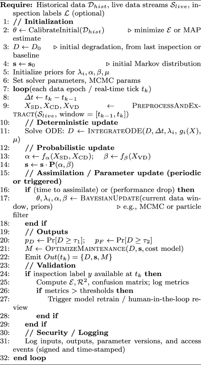
Continuous Digital Twin (DT) Instantiation and Update Loop

Data categorization

Data Categorization plays a crucial role in identifying and notifying relevant stakeholders about abnormal occurrences in real time, particularly in the context of YOLO-based object detection and road infrastructure monitoring. Edge computing acts as an intermediary between the physical layer, where data is collected through IoT devices and cameras, and the cloud layer. Its primary function is to enable immediate detection and response to road infrastructure anomalies. As data, including both physical measurements and visual inputs, is securely transmitted from the physical layer to the cloud, edge computing utilizes a YOLO-based object detection technique to identify irregularities in road conditions. This includes detecting cracks, potholes, faded lane markings, debris, or other structural anomalies in real-time. By processing visual data locally at the edge, edge computing ensures that potential hazards are identified promptly without the need for high-latency cloud processing. Once the edge platform detects any abnormal occurrences, such as significant structural damage or potential safety risks, it immediately triggers alerts and notifications to the appropriate road maintenance teams or authorities. This enables timely intervention and the implementation of corrective measures to maintain road safety and functionality. Edge computing’s real-time response capabilities are critical in road infrastructure monitoring, as they allow for a proactive and efficient approach to managing road conditions. By promptly notifying stakeholders about potential risks or failures, edge computing minimizes downtime, enhances road safety, and prevents further deterioration. This immediate and localized processing ensures a reliable and scalable solution for infrastructure management, leveraging YOLO-based object detection to provide accurate and actionable insights.

Anomaly detection

The proposed study leverages the YOLO model for comprehensive road infrastructure analysis and classification. The YOLO model is specifically chosen for its ability to perform real-time object detection with high accuracy and efficiency, making it particularly suitable for monitoring dynamic and complex environments like road networks. In this study, the YOLO model is applied to analyze visual data captured from smart cameras and other IoT devices deployed across road infrastructure. The model is trained and fine-tuned to detect and classify various road anomalies, including cracks, potholes, faded lane markings, debris, and other structural irregularities. By processing images in a single forward pass, the YOLO model ensures that infrastructure conditions are assessed in real-time, enabling rapid identification of potential hazards. The classification capabilities of the YOLO model go beyond mere detection; it categorizes anomalies based on their severity and type, providing actionable insights for maintenance teams and decision-makers. For instance, the model can differentiate between minor surface cracks and severe structural damage, allowing for prioritized interventions. Additionally, the YOLO model’s ability to process high-resolution images ensures that even small-scale anomalies are accurately detected, contributing to the overall reliability of the analysis.

YOLO-based classification framework with customized technical formulation

Assumptions and indices Let the input image be partitioned into $S\times S$ grid cells. Each cell $i\in \{1,\dots ,S^2\}$ predicts B bounding-box candidates indexed by $b\in \{1,\dots ,B\}$. Let C denote the number of semantic classes. Define the total number of predictions $N:=S^2 B$. The following notation is used for prediction (i, b):

$$\begin{aligned} b_{i,b} = \big (x_{i,b},\,y_{i,b},\,w_{i,b},\,h_{i,b}\big ), \hat{b}_{i,b} = \big (\hat{x}_{i,b},\,\hat{y}_{i,b},\,\hat{w}_{i,b},\,\hat{h}_{i,b}\big ), \end{aligned}$$

where (x, y) are center coordinates relative to the grid cell, and (w, h) are width and height normalized to the image size. Let $\hat{C}_{i,b}\in [0,1]$ denote the predicted confidence for (i, b) and $\hat{P}_{i,b}(c)\in [0,1]$ the predicted conditional class probability $P(c\mid \text {object})$ (so the per-box class score equals $\hat{P}_{i,b}(c)\,\hat{C}_{i,b}$). Assignment indicators:

$$\begin{aligned} \mathbb {1}_{i,b}^{\textrm{obj}} = {\left\{ \begin{array}{ll} 1, & \text { if prediction } (i,b) \text { is assigned to an object },\\ 0, & \text {otherwise}, \end{array}\right. } \end{aligned}$$

Per-box class score For class $c\in \{1,\dots ,C\}$ the final score for box (i, b) is

$$\begin{aligned} \text {score}_{i,b}(c) \;=\; \hat{P}_{i,b}(c)\,\hat{C}_{i,b}. \end{aligned}$$

Customized loss function (modifications)

The proposed total loss is

$$\begin{aligned} \mathcal {L}_{\textrm{total}} = \lambda _{\textrm{loc}}\mathcal {L}_{\textrm{loc}} + \lambda _{\textrm{conf}}\mathcal {L}_{\textrm{conf}} + \lambda _{\textrm{cls}}\mathcal {L}_{\textrm{cls}}, \end{aligned}$$

with tunable scalar weights $\lambda _{\textrm{loc}},\lambda _{\textrm{conf}},\lambda _{\textrm{cls}}>0$ and an additional no-object weight $\lambda _{\textrm{noobj}}>0$ appearing in $\mathcal {L}_{\textrm{conf}}$ below.

Localization loss (for boxes responsible for objects):

$$\begin{aligned} & \mathcal {L}_{\textrm{loc}} = \sum _{i=1}^{S^2}\sum _{b=1}^{B}\mathbb {1}_{i,b}^{\textrm{obj}} \Big [ (x_{i,b}-\hat{x}_{i,b})^2 + (y_{i,b}-\hat{y}_{i,b})^2 + Y] \\ & Y= \big (\sqrt{w_{i,b}}-\sqrt{\hat{w}_{i,b}}\big )^2 + \big (\sqrt{h_{i,b}}-\sqrt{\hat{h}_{i,b}}\big )^2 \Big ]. \end{aligned}$$

(The $\sqrt{\cdot }$ terms stabilize gradients for scale.) Confidence loss (object / no-object weighting).

$$\begin{aligned} \mathcal {L}_{\textrm{conf}} = \sum _{i=1}^{S^2}\sum _{b=1}^{B}\Big [ \mathbb {1}_{i,b}^{\textrm{obj}}(\hat{C}_{i,b}-C_{i,b})^2 + \lambda _{\textrm{noobj}}\mathbb {1}_{i,b}^{\textrm{noobj}}(\hat{C}_{i,b}-C_{i,b})^2 \Big ], \end{aligned}$$

where $C_{i,b}=P(\text {object})\cdot \textrm{IoU}(b_{i,b},b^{\textrm{gt}})$ for the assigned ground-truth box $b^{\textrm{gt}}$ (or $C_{i,b}=0$ when no object). Confidence loss (with WIoU replacement). When WIoU is used, replace $\textrm{IoU}$ by $\textrm{WIoU}$ in the definition of $C_{i,b}$. Classification loss (asymmetric weighting, label smoothing). A weighted cross-entropy with label smoothing is recommended to address class imbalance and calibration:

$$\begin{aligned} \mathcal {L}_{\textrm{cls}} = -\sum _{i=1}^{S^2}\sum _{b=1}^{B}\mathbb {1}_{i,b}^{\textrm{obj}} \sum _{c=1}^{C} w_c\,\tilde{y}_{i,b}(c)\,\log \big (\hat{P}_{i,b}(c)\big ), \end{aligned}$$

where $w_c>0$ is a per-class weight (higher for under-represented defect classes) and $\tilde{y}_{i,b}(\cdot )$ are smoothed one-hot labels:

$$\begin{aligned} \tilde{y}_{i,b}(c^\star )=1-\epsilon ,\qquad \tilde{y}_{i,b}(c)=\frac{\epsilon }{C-1}\ \text { for } c\ne c^\star , \end{aligned}$$

with $c^\star$ the ground-truth class and $\epsilon \in [0,1)$ the label-smoothing parameter. A convenient, tunable penalty is

$$\begin{aligned} \textrm{Penalty}(\delta ) = \exp \big (-\kappa \,\delta ^2\big ),\qquad \kappa >0, \end{aligned}$$

so that small center offsets incur mild penalties while large offsets reduce WIoU more strongly.

Class schema and asymmetric weighting

Four output classes are used:

$$\begin{aligned} \mathcal {C}=\{\textsf {Apt},\ \textsf {Inapt (Crack)},\ \textsf {Inap (Pothole)},\ \textsf {Inap (Other)}\}. \end{aligned}$$

Class imbalance is addressed by setting per-class weights $w_c$ in $\mathcal {L}_{\textrm{cls}}$ (e.g., $w_{\text {Apt}}< w_{\text {Inap (Pothole)}}$). The vector $w=(w_1,\dots ,w_C)$ is a hyperparameter to be tuned (via validation or inverse-frequency heuristics).

Training pipeline modifications

The training pipeline incorporates only the following targeted enhancements (standard YOLO training details omitted):

• Data augmentation Mosaic, CutMix, random cropping/scaling, photometric jitter; ensure augmentations preserve geometric consistency for bounding boxes.

• Label smoothing Smoothing parameter $\epsilon$ as above to improve calibration.

• Class imbalance handling per-class weights $w_c$ in classification loss or focal-loss replacement:

  $$\begin{aligned} \mathcal {L}_{\textrm{focal}} = -\sum _{i,b}\sum _{c} \mathbb {1}_{i,b}^{\textrm{obj}}\,w_c\,(1-\hat{P}_{i,b}(c))^\gamma \,\tilde{y}_{i,b}(c)\log \hat{P}_{i,b}(c), \end{aligned}$$

  with focusing parameter $\gamma \ge 0$ (optional).

• Confidence target Use $\textrm{WIoU}$ for $C_{i,b}$ when greater robustness to center error is required.

• Optimizer & scheduling Standard choices (SGD with momentum or AdamW), cosine or step LR schedule; hyperparameters selected via validation.

Algorithm 2

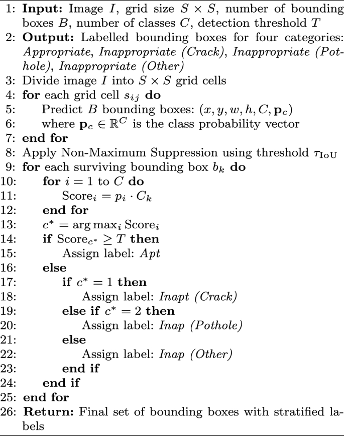
Enhanced YOLO Classification with Custom Label Stratification and Threshold Adaptation

Data mining

Spatial Mining is utilized in road infrastructure analysis to extract and consolidate data across geographical regions based on predefined spatial criteria. The proposed framework is responsible for retrieving spatially distributed data from cloud storage systems. This approach is particularly suited for road infrastructure analysis, as various datasets, such as traffic patterns, road conditions, and environmental factors, are stored with spatial attributes. Spatial mining facilitates data abstraction, enabling the generation of valuable insights by analyzing data from multiple geographical perspectives. This is critical because road infrastructure conditions vary across locations, and capturing spatial diversity is essential. For instance, some events, like monitoring traffic flow or weather conditions, may require high-resolution spatial data, while others, such as detecting road damage or construction activities, may only need localized or regional data. The proposed technique abstracts road infrastructure data using Spatial Patterns, which enables the identification of meaningful patterns and relationships within spatially structured datasets stored in the cloud. By leveraging spatial mining techniques, the proposed model can uncover insights that might not be apparent through non-spatial or static data analysis. The ability to effectively retrieve and analyze spatially structured road infrastructure data from cloud storage is a crucial component of the overall framework, as it provides the foundation for advanced processing and decision-making in subsequent layers, such as predictive maintenance or traffic optimization.

Definition 1

(Spatial Segment) A Spatial Segment in road infrastructure analysis is defined as a set of attributes $(R_l, S_l)$, where $R_l$ represents a road infrastructure attribute (e.g., road condition, traffic density), and $S_l$ corresponds to a fixed spatial region $\delta S$. Here, $(R_l, S_l)$ denotes the attribute $R_l$ captured by IoT sensors or monitoring devices within the spatial region $\delta S$. Mathematically, it is represented as:

$$\begin{aligned} {[}R_1, S_1], [R_2, S_2], \dots , [R_l, S_l]. \end{aligned}$$

Definition 2

(Spatial extraction) Spatial Extraction refers to the technique used for abstracting data from structured road infrastructure datasets. It is represented as:

$$\begin{aligned} {[}R_{ab}, R_{ap}], \end{aligned}$$

where $R_{ab}$ is the abstraction function, and $R_{ap}$ represents the implication of abstraction for a specific spatial segment.

Fig. 5

Spatial extraction procedure.

Key advantages of spatial mining

• Localized insights Enables the identification of specific regions requiring maintenance or optimization, such as areas with high traffic congestion or frequent road damage.

• Scalability Facilitates the analysis of large-scale road networks by dividing them into manageable spatial segments.

• Integration with IoT Leverages IoT-enabled devices to continuously monitor and update spatial data, ensuring real-time analysis and decision-making.

• Enhanced decision-making Provides the foundation for advanced applications, such as predictive maintenance, route optimization, and resource allocation.

Mathematical representation of spatial mining

The mathematical representation of spatial mining in road infrastructure analysis is as follows:

Spatial segment representation Each spatial segment is defined as:

$$\begin{aligned} S = \{(R_1, S_1), (R_2, S_2), \dots , (R_n, S_n)\}, \end{aligned}$$

Where $R_i$ represents the road attribute (e.g., road condition, traffic density) and $S_i$ represents the spatial region.

Spatial abstraction function The abstraction function $R_{ab}$ is defined as:

$$\begin{aligned} R_{ab}(S) = \int _{S} f(R, S) \, dS, \end{aligned}$$

Where $f(R, S)$ represents the relationship between the road attribute $R$ and the spatial region $S$, and the integral aggregates the data over the spatial region.

Spatial data aggregation Spatial data aggregation is represented as:

$$\begin{aligned} R_{agg} = \sum _{i=1}^n R_i(S_i), \end{aligned}$$

Where $R_{agg}$ is the aggregated road attribute across all spatial segments. By leveraging spatial mining techniques, the proposed framework enables the effective analysis of road infrastructure data across geographical regions. This approach facilitates localized insights, scalability, and integration with IoT systems, providing the foundation for advanced decision-making in road infrastructure management.

Decision making

Decision-making is employed to predict potential vulnerabilities in road infrastructure. The primary objective is to identify instances where sections of the infrastructure may be at risk due to structural, environmental, or traffic-related factors. By leveraging a hybrid deep learning framework, the proposed system aims to enhance prediction accuracy and reliability. This hybrid approach integrates multiple deep learning architectures to analyze diverse data streams collected from IoT-enabled systems, including environmental sensors, traffic monitoring devices, and structural health monitoring systems. These data streams capture critical information about road conditions, traffic patterns, and environmental factors. Through the combination of deep learning models, the framework is better equipped to identify complex, interdependent patterns that contribute to infrastructure vulnerabilities. For instance, it can detect sudden changes in traffic density, abnormal vibration patterns, or environmental conditions (e.g., extreme weather) that may adversely affect road infrastructure.

Road anomaly assessment

The proposed hybrid deep learning approach for assessing road infrastructure anomalies as represented in Fig. 5, focuses on accurately identifying characteristics that indicate structural or operational risks. The framework utilizes Convolutional Neural Networks (CNNs) to process IoT sensor data collected from the road network over the DT platform. These CNNs are trained to extract features related to potential vulnerabilities and predict their severity levels. The CNN module comprises convolutional and pooling layers, where convolutional layers apply multiple filters to recognize local patterns in raw data signals, and pooling layers summarize these patterns. This architecture enables real-time feature extraction and analysis, improving the system’s ability to identify relevant indicators of road infrastructure risks. However, CNNs alone may struggle to capture long-term temporal dependencies, especially when dealing with extended patterns of traffic flow or structural stress. To address this limitation, the proposed hybrid framework incorporates Gated Recurrent Units (GRUs), a type of Recurrent Neural Network (RNN) designed to model sequential and time-dependent data effectively. GRUs enhance the system’s ability to analyze time-series data, enabling it to learn from complex temporal patterns associated with infrastructure vulnerabilities. By combining CNNs and GRUs, the hybrid framework leverages the strengths of both architectures, resulting in a robust and comprehensive system for predicting potential anomalies.

CNN-BiGRU architecture for infrastructure anomaly detection

The proposed CNN-BiGRU architecture integrates spatial feature extraction and temporal sequence modeling to enhance road infrastructure anomaly detection, as shown in Fig. 6. The CNN module extracts discriminative spatial features from input data, which are then sequentially modeled using a bidirectional GRU (BiGRU) to capture temporal dependencies. This hybrid framework improves detection accuracy, particularly when the training data is limited.

The CNN module processes input images of size $128 \times 128 \times 3$, applying three convolutional blocks. Each block comprises:

• A 2D convolutional layer with kernel size $3 \times 3$, stride 1, and padding 1,

• ReLU activation,

• Batch Normalization for stable training,

• Max-pooling layer with size $2 \times 2$.

The output of the CNN is a feature matrix:

$$\begin{aligned} F = [f(1), f(2), \dots , f(n)], \end{aligned}$$

where each $f(i) \in \mathbb {R}^{d}$ represents the feature vector at timestep $i$, fed into the BiGRU for sequential modeling. The GRU module includes two stacked bidirectional GRU layers, each with 128 hidden units per direction (total 256), using hyperbolic tangent ($\tanh$) as the activation and sigmoid ($\sigma$) for the gates.

GRU dynamics

$$\begin{aligned} \begin{aligned} r(t)&= \sigma (W_r f(t) + U_r h(t-1) + b_r), \\ z(t)&= \sigma (W_z f(t) + U_z h(t-1) + b_z), \\ \tilde{h}(t)&= \tanh (W_h f(t) + U_h [r(t) \odot h(t-1)] + b_h), \\ h(t)&= z(t) \odot h(t-1) + (1 - z(t)) \odot \tilde{h}(t)). \end{aligned} \end{aligned}$$

The final GRU output $H = [h(1), h(2), \dots , h(n)]$ is flattened and passed through a Multilayer Perceptron (MLP) with:

• Dropout layer ($p = 0.5$) to prevent overfitting,

• Dense layer with 64 units and ReLU activation,

• Output dense layer with 4 units (class labels).

Softmax prediction

$$\begin{aligned} P(t) = \text {Softmax}(W_o h(t) + b_o) \end{aligned}$$

Loss function Weighted categorical cross-entropy is used:

$$\begin{aligned} \mathcal {L}_{\text {cls}} = - \sum _{i=1}^{C} w_i \cdot Y_i(t) \cdot \log (P_i(t)) \end{aligned}$$

where $w_i$ are inverse-frequency class weights.

Training settings The network is trained using the Adam optimizer (learning rate $0.001$), batch size 32, and early stopping based on validation loss.

Data augmentation CutMix, Mosaic, and label smoothing are employed to enhance robustness.

Fig. 6

CNN-BiGRU architecture for road infrastructure anomaly detection.

Experimental simulation

This section evaluates the performance of the proposed road infrastructure monitoring system in predicting and analyzing anomalies. The framework consists of four main components: data acquisition, edge-layer anomaly detection (YOLOv11), spatial data mining, and CNN-BiGRU-based predictive decision-making.

Dataset description and integration

The LiRA-CD (Linked Infrastructure for Road Analysis—Condition Dataset)³⁵ and UCI environmental dataset were used. The LiRA-CD dataset contains approximately 38,000 annotated images, including:

• Potholes 9420 instances,

• Cracks 12,870 instances,

• Rutting 7610 instances,

• Surface wear 8100 instances.

Annotations follow COCO-style polygon labeling. YOLOv11 was trained exclusively on these image annotations to detect and localize surface damage. In contrast, the CNN-BiGRU model processes the numerical sensor and contextual features (e.g., vibration, strain, temperature, humidity, traffic load), not raw images. The output from YOLOv11 (e.g., bounding box frequency, damage area ratio) is aggregated into feature vectors and supplied as auxiliary input to the CNN-BiGRU for joint analysis with time-series sensor data. Hence, the two models operate in a complementary but modular pipeline rather than a single jointly-trained network. The UCI environmental dataset provides 30,021 time-series samples, augmenting the context for environmental and temporal correlation modeling.

Training configuration

The dataset was split 70:15:15 for training, validation, and testing using stratified sampling across both spatial and temporal segments. Cross-validation (5-fold) was also conducted for robustness. The YOLOv11 model was trained on images, while the CNN-BiGRU model was trained on numerical sensor features and YOLO-derived metadata.

Model training and evaluation

The models were trained using AdamW with an initial learning rate of 0.001. The performance was assessed using mAP, AUROC, F1-score, and $r^2$ metrics. The modular design allows independent optimization of detection and predictive components while maintaining synchronized data flow for real-time deployment.

Data categorization efficacy

The performance of the proposed YOLO-based classifier for road infrastructure monitoring was rigorously evaluated using standard object detection metrics: mean Average Precision at IoU threshold 0.5 (mAP@0.5), mean Average Precision averaged over IoU thresholds from 0.5 to 0.95 in steps of 0.05 (mAP@0.5:0.95), per-class precision and recall, and Area Under the Receiver Operating Characteristic Curve (AUROC). These metrics provide a comprehensive understanding of detection accuracy, localization quality, and class-wise robustness.

Road condition dataset performance

Table 3 summarizes the performance of the proposed model and baseline state-of-the-art detectors on the road condition dataset.

Table 3 Detection performance on road condition dataset.

Per-class evaluation revealed consistently high precision and recall across surface defects, potholes, road roughness, and faded markings. The proposed model achieved per-class AUROC exceeding 0.97 across all categories, indicating exceptional separability between positive and negative cases even in noisy urban environments.

Environmental dataset performance

Table 4 presents detection accuracy on environmental sensor-derived datasets.

Table 4 Detection performance on environmental dataset.

The proposed model demonstrated superior performance across all detection dimensions, particularly in high-resolution data from heterogeneous sensors. mAP@0.5:0.95 scores indicate strong localization performance even under varied occlusions and lighting. AUROC values further confirm the robustness of binary and multi-class separation under real-world uncertainty. The adoption of modern detection metrics highlights the superiority of the proposed YOLO-based framework over state-of-the-art detectors. It consistently achieves higher precision, recall, and AUROC, ensuring accurate and reliable road infrastructure intelligence.

Prediction efficacy assessment

Performing real-time analysis of datasets for evaluating road infrastructure conditions presents significant challenges in terms of prediction efficiency. As previously mentioned, the datasets being analyzed contain substantial volumes of data related to various road attributes. Therefore, it is critical to assess the accuracy and reliability of the prediction models employed. Before conducting the prediction analysis, these diverse datasets are consolidated into a unified format to ensure consistency in evaluation. To evaluate the efficiency and performance of the prediction process, several statistical metrics are utilized. Specifically, three key statistical measures are calculated:

Table 5 Performance comparison of the proposed model and previous studies in terms of $r^2$, AAE, and ASE.

Average square error (ASE)

This metric quantifies the average squared difference between the predicted values $\hat{y}_i$ and the actual values $y_i$. Mathematically, it is expressed as:

$$\begin{aligned} ASE = \frac{1}{n} \sum _{i=1}^n (\hat{y}_i - y_i)^2 \end{aligned}$$

Where $n$ is the total number of data points.

Pearson’s correlation coefficient ($r^2$)

This statistic measures the linear correlation between the predicted values $\hat{y}_i$ and the actual values $y_i$, providing insight into the strength of the relationship.

Average absolute error (AAE)

This measure calculates the average of the absolute differences between the predicted values $\hat{y}_i$ and the actual values $y_i$, reflecting the overall prediction accuracy. These statistical parameters are essential for assessing the overall accuracy and effectiveness of the proposed prediction model.

Performance evaluation

To evaluate the performance of the proposed prediction models, three state-of-the-art approaches were considered Rathee et al.³⁸, Zhang et al.³⁷, and Luo et al.³⁶. It is important to note that only the prediction models were varied during the evaluation, while the rest of the system remained unchanged. The results of the experimental evaluation are summarized in Table 5.

Key results

According to the results, the proposed model significantly outperformed previous studies by Rathee et al.³⁸, Zhang et al.³⁷, and Luo et al.³⁶ in terms of Pearson’s correlation coefficient ($r^2$). The proposed model achieved a value of approximately 0.77 (SD 0.77), indicating a strong correlation between the predicted and actual road conditions. In comparison, Rathee et al.³⁸ obtained a lower $r^2$ value of 0.67 (SD 0.73), while Zhang et al.³⁷ and Luo et al.³⁶ recorded even lower values of 0.57 (SD 0.17) and 0.50 (SD 0.11), respectively. This demonstrates that the proposed model not only surpasses these existing approaches but also provides a more reliable representation of the relationship between predicted and actual conditions. In terms of Average Absolute Error (AAE), the proposed model further demonstrated superior performance, achieving an AAE of 0.31 (SD 0.01). This is a stark contrast to the results from Rathee et al.³⁸, which reported an AAE of 0.71 (SD 0.04), and Zhang et al.³⁷ with an AAE of 0.73 (SD 0.08). Luo et al.³⁶ also fell short with an AAE of 0.75 (SD 0.59). The lower AAE of the proposed model indicates its greater accuracy in predicting road conditions, minimizing the average deviation from actual measurements. Furthermore, regarding the Average Square Error (ASE), the proposed model achieved better results with a value of 0.34 (SD 0.13). In contrast, Rathee et al.³⁸ recorded an ASE of 0.78 (SD 0.85), while Zhang et al.³⁷ and Luo et al.³⁶ showed ASE values of 0.68 (SD 0.28) and 0.78 (SD 0.89), respectively. The reduced ASE of the proposed model signifies its enhanced predictive capability and reliability. Based on these findings, it can be concluded that the proposed CNN-BiGRU model is highly accurate and effective for predicting road infrastructure conditions. Its ability to outperform existing state-of-the-art approaches highlights its potential as a reliable tool for real-time road condition monitoring and maintenance planning. This advancement not only contributes to the field of infrastructure management but also supports the development of smarter, more responsive transport systems.

Fig. 7

Temporal efficiency.

Real-time mining efficiency

The proposed real-time framework for automated road infrastructure condition analysis is composed of three primary modules:

• 1. YOLO-based classification A quantized YOLOv11-based classifier categorizes raw road imagery and sensor streams into predefined defect classes (e.g., potholes, cracks, faded markings).

• 2. Data mining Time-series road and environmental data are dynamically retrieved from a cloud-based repository hosted on Amazon EC2.

• 3. Severity prediction A lightweight CNN-BiGRU hybrid model is used to forecast the Infrastructure Severity Index (ISI), representing the road segment’s degradation risk.

Figure 7 presents the detailed results.

Temporal efficiency

The total latency is defined as:

$$\begin{aligned} T_{\text {total}} = T_{\text {classification}} + T_{\text {mine}} + T_{\text {prediction}} \end{aligned}$$

where:

• $T_{\text {classification}}$: YOLO-based image classification latency

• $T_{\text {mine}}$: Road/environmental data extraction time from cloud

• $T_{\text {prediction}}$: ISI prediction time using CNN-BiGRU

The evaluation was conducted on a Raspberry Pi 4 (8 GB RAM, 2.12 GHz ARM Cortex-A72 CPU), with the following inference configuration:

• Input resolution $416 \times 416$ pixels (downsampled dynamically from original video frames)

• Batch size 1 (real-time frame-by-frame inference)

• Quantization Post-training 8-bit INT quantization using TensorRT for YOLO and CNN layers

• Threading Multi-threaded inference pipeline leveraging 4-core parallelism using Python multiprocessing and OpenMP backend

• Throughput Sustained 105 FPS under continuous inference with thermal throttling mitigation

Road condition dataset evaluation

The average measured latency breakdown is as follows:

$$\begin{aligned} \begin{aligned} T_{\text {mine}}&= 3.2\, \text {ms} \\ T_{\text {classification}}&= 4.3\, \text {ms} \\ T_{\text {prediction}}&= 2.0\, \text {ms} \\ T_{\text {total}}&= 9.5\, \text {ms} \end{aligned} \end{aligned}$$

This low latency ensures that the system can process more than 100 frames per second, making it suitable for real-time embedded deployment in smart transportation applications.

Environmental dataset evaluation

For environmental sensor analysis:

$$\begin{aligned} \begin{aligned} T_{\text {mine}}&= 2.9\, \text {ms} \\ T_{\text {classification}}&= 3.8\, \text {ms} \\ T_{\text {prediction}}&= 1.9\, \text {ms} \\ T_{\text {total}}&= 8.6\, \text {ms} \end{aligned} \end{aligned}$$

These results confirm that the proposed architecture achieves sub-10 millisecond end-to-end inference latency on edge hardware. The YOLOv11 classifier benefits from spatial-to-depth optimization and quantization, enabling high-speed object localization. Simultaneously, the CNN-BiGRU predictor provides temporal robustness while maintaining computational tractability. Together, the pipeline delivers real-time severity estimation for road segments, facilitating timely alerts and predictive maintenance strategies. The latency-performance trade-off was optimized without sacrificing accuracy, ensuring operational viability in resource-constrained environments.

Stability analysis

The stability of the proposed road infrastructure analysis system was examined to evaluate its reliability under varying data conditions and fluctuating input distributions. Since the severity analysis task involves processing heterogeneous and large-scale datasets, it is essential to verify that the system maintains consistent performance despite changes in input data characteristics. To quantitatively assess stability, the Mean Absolute Shift (MAS) metric is employed. MAS measures the average absolute deviation of the system’s outputs relative to their mean values across multiple iterations or input variations. A lower MAS value indicates higher system stability, as it reflects smaller deviations and more consistent performance. Conversely, a higher MAS value implies greater output variability and reduced stability.

Fig. 8

Stability analysis of the proposed system across multiple datasets.

The MAS is mathematically defined as:

$$\begin{aligned} \text {MAS} = \frac{1}{n} \sum _{i=1}^{n} |x_i - \bar{x}|, \end{aligned}$$

where:

• $x_i$ represents individual output measurements,

• $\bar{x}$ denotes the mean of the outputs,

• $n$ is the total number of samples or iterations.

As illustrated in Fig. 8, the proposed system achieved an average MAS value of approximately $0.51$, signifying low deviation and strong operational stability across diverse datasets. The minimal MAS variation demonstrates that the model can process fluctuating or noisy input data without notable degradation in predictive performance. This finding highlights the robustness of the proposed framework, particularly when applied to large-scale and heterogeneous road infrastructure datasets. The stability evaluation complements the earlier performance analysis, confirming that the integration of YOLO-based detection, CNN-BiGRU severity estimation, and Digital Twin contextual modeling ensures consistent and reliable operation in real-world deployment scenarios.

Ablation study

An ablation study was performed to quantify the contribution of each core component-Digital Twin (DT) contextual modeling, YOLO-based anomaly classification, and CNN-BiGRU-based severity prediction-toward the overall system performance. The objective was to determine how these modules individually and collectively influence detection accuracy, temporal consistency, and computational efficiency. All experiments were conducted on the LiRA-CD road condition and UCI environmental datasets with an input resolution of 640$\times$640, batch size of 16, and 8-bit quantized inference on a Jetson Xavier NX with TensorRT acceleration.

Experimental setup

Four model configurations were evaluated:

• 1. Baseline (No DT, Basic Classifier, MLP Predictor): A minimal configuration using handcrafted statistical features and a multilayer perceptron (MLP) for severity prediction. This served as a reference for evaluating the contribution of deep learning and contextual modeling.

• 2. YOLO + MLP (No DT): YOLOv11 was introduced for visual object detection, replacing the handcrafted feature classifier. The MLP remained as the severity predictor, isolating the impact of visual feature extraction.

• 3. YOLO + CNN-BiGRU (No DT): The MLP was replaced with the CNN-BiGRU module to introduce temporal modeling of sensor data while retaining YOLO for spatial feature extraction. This configuration assesses the role of sequential learning in capturing time-dependent degradation patterns.

• 4. Proposed Full Pipeline (DT + YOLO + CNN-BiGRU): The complete framework integrating DT-based contextual modeling with YOLOv11 and CNN-BiGRU to provide multimodal spatio-temporal inference and environmental awareness.

Quantitative results

Table 6 summarizes the quantitative outcomes of the ablation study.

Table 6 Ablation study results on road condition dataset.

Results and discussion

Table 6 indicates a consistent and incremental improvement across all performance metrics as additional modules are integrated into the pipeline.

• YOLO integration The introduction of YOLOv11 led to a substantial performance increase of 13.42% in mAP@0.5 compared to the baseline, demonstrating its effectiveness in accurately localizing and classifying visible infrastructure anomalies. The precision improvement is attributed to YOLOv11’s multi-scale feature extraction and anchor-free detection, which reduces false detections on small or partially occluded defects.

• Temporal modeling via CNN-BiGRU Replacing the MLP with CNN-BiGRU provided an additional 3.6% gain in AUROC and improved temporal coherence in severity estimation. The GRU’s recurrent gating mechanism enabled the model to capture degradation progression over time, enhancing reliability in sequential prediction tasks.

• DT contextualization Incorporating the Digital Twin module further improved mAP@0.5 by 2.25% and yielded the highest F1-score (0.925). This improvement results from the DT’s ability to assimilate environmental parameters-such as humidity, temperature, and vibration intensity-into the prediction process, allowing the model to account for contextual variability that directly affects structural health.

Overall, the ablation results confirm that each component contributes uniquely: YOLOv11 enhances spatial detection accuracy, CNN-BiGRU captures temporal dependencies, and the DT layer enriches contextual awareness. The integration of all three achieves the best balance between detection precision, temporal stability, and real-time inference performance.

Class distribution analysis and impact of imbalance

A critical aspect of evaluating the robustness of any detection and prediction framework lies in understanding the distribution of classes within the dataset. For the LiRA-CD dataset (road anomalies) and the UCI environmental dataset, preliminary inspection reveals that the data is not uniformly distributed across anomaly categories. For example, minor surface cracks and faded markings constitute the majority of annotated instances, whereas severe potholes, large-scale structural fractures, or snow-covered road conditions are comparatively underrepresented.

Observed class distribution

Table 7 provides an illustrative breakdown of the dataset distribution across major anomaly types. Although exact proportions may vary depending on the recording session and environment, the general pattern indicates class imbalance.

Table 7 Illustrative class distribution in LiRA-CD dataset.

Per-class statistical performance

Table 8 summarizes the proposed model’s per-class detection and classification results. As expected, the majority of classes, such as surface cracks and faded markings achieve higher precision and recall, while rare classes (severe structural damage, snow/ice covered roads) exhibit degraded performance.

Table 8 Per-class detection and classification results of the proposed model.

Confusion matrix analysis

To further examine model behavior under class imbalance, the normalized confusion matrix in Table 9 provides detailed insights into class-specific misclassifications. While the majority of classes, such as Surface Cracks and Faded/Missing Markings, show strong diagonal dominance, rare categories such as Snow/Ice Covered Roads exhibit higher off-diagonal errors, indicating confusion with faded markings and potholes.

Table 9 Normalized confusion matrix of proposed model.

Impact of imbalance on performance

The observed imbalance has direct implications for both object detection (YOLOv11) and sequential prediction (CNN-BiGRU):

• Bias toward frequent classes The model tends to favor the detection of cracks and faded markings due to their higher prevalence, potentially leading to inflated average accuracy but poor sensitivity to rare yet critical classes.

• Reduced recall for rare events Severe potholes and snow-covered conditions, despite being safety-critical, may exhibit high false-negative rates due to insufficient training samples.

• Temporal prediction skew In the CNN-BiGRU stage, recurrent dynamics are dominated by majority-class patterns, limiting the model’s ability to generalize over underrepresented anomalies.

Mitigation strategies

To counteract the adverse effects of imbalance, the following strategies are suggested:

• 1. Data augmentation Employing GAN-based synthetic sample generation for rare anomaly types and standard augmentation (rotation, noise injection, color jitter) for balanced representation.

• 2. Cost-sensitive learning Applying weighted cross-entropy or focal loss functions to penalize misclassifications of rare classes more heavily.

• 3. Balanced sampling Enforcing stratified batch composition during training to maintain consistent representation across all anomaly categories.

• 4. Per-class evaluation Reporting per-class precision, recall, F1, and AUROC alongside aggregate metrics to reflect the true performance across all severity levels.

Implications for deployment

In real-world deployments, rare but severe anomalies (e.g., large potholes, structural failures) are often the most consequential. Failure to account for dataset imbalance may result in models that perform well on average but fail in mission-critical scenarios. Therefore, explicit monitoring of class distribution and the adoption of imbalance-aware learning strategies are essential for developing robust and reliable road infrastructure monitoring systems.

Limitations

Despite the promising results achieved by the proposed framework in real-time road infrastructure monitoring, several limitations remain that warrant further investigation:

• Data domain bias The model performance is highly dependent on the geographical and environmental characteristics of the training datasets (e.g., LiRA-CD and UCI). As a result, generalization to other cities, climates, or road types may be limited unless domain adaptation techniques are applied.

• Limited multimodal fusion Although road condition and environmental data are analyzed in parallel, the framework currently treats these modalities independently. This limits the model’s ability to capture cross-modal dependencies (e.g., how humidity influences pothole formation over time).

• Edge hardware constraints Real-time deployment is optimized for low-power devices (e.g., Raspberry Pi), which limits the complexity and depth of neural models. Consequently, accuracy may be slightly compromised compared to models running on high-performance GPUs.

• Weather and lighting variability The YOLO-based classifier may underperform under extreme lighting or adverse weather conditions (e.g., glare, shadows, heavy rain), which are not extensively covered in the training data.

  • Lighting variability The model exhibits reduced accuracy under extreme lighting conditions such as low-light (night-time) or overexposed scenarios (e.g., direct sunlight glare). Although YOLOv11 incorporates data augmentation strategies (e.g., brightness jittering), significant visual degradation can impair feature extraction, leading to false positives or missed detections, particularly for faint or small-scale road defects.

  • Weather-induced noise Adverse weather conditions-such as rain, snow, or fog-introduce noise in both visual and sensor inputs. Snow-covered roads may occlude surface features, while precipitation introduces reflection artifacts. The model’s sensitivity to such artifacts can reduce classification reliability, especially in multi-class scenarios where classes share subtle boundary characteristics.

  • Sensor noise and occlusions The CNN-BiGRU module processes time-series sensor data; however, real-world IoT streams are susceptible to packet loss, calibration drift, or hardware faults. Although temporal filtering partially mitigates this issue, extended missing sequences or anomalous spikes in data can degrade the severity index prediction performance.

  • Domain shift and generalization The model is trained on the LiRA-CD dataset, which reflects specific urban/highway conditions in Copenhagen. Generalizing to different geographic regions with distinct pavement types, road markings, or vehicle sensor configurations (e.g., camera angles or resolution) may require transfer learning or domain adaptation.

  • Edge resource constraints While the model demonstrates real-time performance on a Raspberry Pi 4, deployment on lower-end edge devices or in battery-constrained settings may necessitate further quantization, pruning, or distillation, potentially at the cost of reduced model accuracy.

  To address these challenges, future work will focus on incorporating multi-sensor fusion (e.g., LiDAR, radar), domain adaptation strategies, and adversarial training for improved resilience under variable lighting and environmental noise. Additionally, active learning techniques could be used to continuously retrain the model using edge-collected edge cases, improving long-term performance in heterogeneous real-world settings.

These limitations present avenues for future research, including the integration of uncertainty-aware models, domain adaptation strategies, self-supervised learning for label-scarce regions, and deployment on heterogeneous IoT networks with dynamic model scaling.

Conclusion

The proposed smart road infrastructure monitoring system demonstrates significant potential in addressing critical challenges related to road safety and operational efficiency. By integrating YOLO with deep learning and leveraging DT technology supported by IoT, the system provides real-time monitoring and simulation capabilities. The CNN-BiGRU model, coupled with a YOLO classification technique, has shown superior performance when validated on a dataset of 60,023 instances. Key results include high temporal efficiency 9.5 ms, classification efficacy (Precision: (96.50%), Sensitivity: (95.29%), Specificity: (96.39%), and F-Measure: (96.19%)), robust decision-making efficiency ($r^2 = 77\%$), minimal error rate (AAE = 0.31, ASE = 0.34), and strong stability. These findings underscore the system’s ability to provide accurate, reliable, and efficient monitoring of road infrastructure. Future research should focus on optimizing network bandwidth to facilitate large-scale deployment and enhancing data security measures to protect sensitive infrastructure information. The proposed system offers a promising pathway for improving the safety and sustainability of road networks globally.

References

Grum, B. et al. Applicability and cost implication of labor-based methods for sustainable road maintenance (SRM) in developing countries. Adv. Civ. Eng. 2023(1), 1–12 (2023).
Sadeghi, P. & Goli, A. Investigating the impact of pavement condition and weather characteristics on road accidents. Int. J. Crashworthiness 29(6), 973–989 (2024).
Miao, Yu. et al. Construction and optimization of asphalt pavement texture characterization model based on binocular vision and deep learning. Measurement 248, 116946 (2025).
Wang, H.-P., Guo, Y.-X., Meng-Yi, W., Xiang, K. & Sun, S.-R. Review on structural damage rehabilitation and performance assessment of asphalt pavements. Rev. Adv. Mater. Sci. 60(1), 438–449 (2021).
Hauashdh, A., Jailani, J., Rahman, I. A. & Al-Fadhali, N. Strategic approaches towards achieving sustainable and effective building maintenance practices in maintenance-managed buildings: A combination of expert interviews and a literature review. J. Build. Eng. 45, 1–13 (2022).
Ijari, K. & Paternina-Arboleda, C. D. Sustainable pavement management: Harnessing advanced machine learning for enhanced road maintenance. Appl. Sci. 14(15), 1–17 (2024).
Solla, M., Pérez-Gracia, V. & Fontul, S. A review of GPR application on transport infrastructures: Troubleshooting and best practices. Remote Sens. 13(4), 1–54 (2021).
Kulambayev, B. et al. Real-time road surface damage detection framework based on mask R-CNN model. Int. J. Adv. Comput. Sci. Appl. 14(9), 1–9 (2023).
Islam, M. S. et al. Advancement in the automation of paved roadways performance patrolling: A review. Measurement 0(232), 1–13 (2024).
Zeng, Y. et al. Prediction of compressive and flexural strength of coal gangue-based geopolymer using machine learning method. Mater. Today Commun. 44, 112076 (2025).
Karim, S. et al. Current advances and future perspectives of image fusion: A comprehensive review. Inf. Fusion 90, 185–217 (2023).
Archana, R. & Jeevaraj, P. S. E. Deep learning models for digital image processing: A review. Artif. Intell. Rev. 57(1), 1–33 (2024).
Xiangyang, X. et al. Crack detection and comparison study based on faster R-CNN and mask R-CNN. Sensors 22(3), 1–17 (2022).
Hacıefendioğlu, K. & Basri Başağa, H. Concrete road crack detection using deep learning-based faster R-CNN method. Iran. J. Sci. Technol. Trans. Civ. Eng. 46(2), 1621–1633 (2022).
Chen, M. et al. Improved faster R-CNN for fabric defect detection based on Gabor filter with genetic algorithm optimization. Comput. Ind. 134, 1–10 (2022).
Amândio, M., Parente, M., Neves, J. & Fonseca, P. Integration of smart pavement data with decision support systems: A systematic review. Buildings 11(12), 1–24 (2021).
Ren, M., Zhang, X., Chen, X., Zhou, B. & Feng, Z. YOLOv5s-m: A deep learning network model for road pavement damage detection from urban street-view imagery. Int. J. Appl. Earth Obs. Geoinf. 120, 1–13 (2023).
Olorunshola, O. E., Irhebhude, M. E. & Evwiekpaefe, A. E. A comparative study of yolov5 and yolov7 object detection algorithms. J. Comput. Soc. Inform. 2(1), 1–12 (2023).
Wei Li, J., Huyan, R. G., Hao, X., Yuanjiao, H. & Zhang, Y. Unsupervised deep learning for road crack classification by fusing convolutional neural network and k_means clustering. J. Transp. Eng. Part B Pavements 147(4), 1–14 (2021).
Jin, C., Kong, X., Chang, J., Cheng, H. & Liu, X. Internal crack detection of castings: A study based on relief algorithm and Adaboost-SVM. Int. J. Adv. Manuf. Technol. 108(9), 3313–3322 (2020).
Sharifuzzaman, S. A. S. M. et al. Bayes R-CNN: An uncertainty-aware Bayesian approach to object detection in remote sensing imagery for enhanced scene interpretation. Remote Sens. 16(13), 1–31 (2024).
Chaudhary, V., Buttar, P. K. & Sachan, M. K. Satellite imagery analysis for road segmentation using U-Net architecture. J. Supercomput. 78(10), 12710–12725 (2022).
Zhao, T. et al. Artificial intelligence for geoscience: Progress, challenges and perspectives. Innovation 1–26 (2024).
Guo, C., Hao, K., Zuo, C. A few-shot road extraction method using customized segment anything model. In 2024 9th International Conference on Intelligent Computing and Signal Processing (ICSP) 1036–1039 (2024).
Luo, X., Liu, R., He, X. & Wang, H. A road damage detection model based on improved RT-DETR for complex environments. IEEE Trans. Instrum. Meas. 74, 1–13 (2025).
Sun, Z., Lingxi Zhu, S., Qin, Y. Y., Ruiwen, J. & Li, Q. Road surface defect detection algorithm based on YOLOv8. Electronics 13(12), 1–13 (2024).
Ji, H., Kim, J., Hwang, S. & Park, E. Automated crack detection via semantic segmentation approaches using advanced u-net architecture. Intell. Autom. Soft Comput. 34(1), 1–15 (2022).
Lin, Q., Li, W., Zheng, X., Fan, H. & Li, Z. DeepCrackAT: An effective crack segmentation framework based on learning multi-scale crack features. Eng. Appl. Artif. Intell. 126, 1–11 (2023).
Dai, Y., Wang, J., Li, J. & Li, J. MDRNet: A lightweight network for real-time semantic segmentation in street scenes. Assem. Autom. 41(6), 725–733 (2021).
Yan, K. & Zhang, Z. Automated asphalt highway pavement crack detection based on deformable single shot multi-box detector under a complex environment. IEEE Access 9, 150925–150938 (2021).
Sami, A. A., Sakib, S., Deb, K. & Sarker, I. H. Improved YOLOv5-based real-time road pavement damage detection in road infrastructure management. Algorithms 16(9), 1–23 (2023).
Yar, H., Khan, Z. A., Ullah, F. U. M., Ullah, W. & Baik, S. W. A modified YOLOv5 architecture for efficient fire detection in smart cities. Expert Syst. Appl. 231, 1–11 (2023).
Feng, Y. et al. A efficient and accurate UAV detection method based on YOLOv5s. Appl. Sci. 14(15), 1–17 (2024).
Li, Y., Yin, C., Lei, Y., Zhang, J. & Yan, Y. RDD-YOLO: Road damage detection algorithm based on improved you only look once version 8. Appl. Sci. 14(8), 1–17 (2024).
Skar, A. et al. LiRA-CD: An open-source dataset for road condition modelling and research. Data Brief 49, 1–15 (2023).
Luo, D., Jianbo, L. & Guo, G. Road anomaly detection through deep learning approaches. IEEE Access 8, 117390–117404 (2020).
Zhang, M. et al. Urban anomaly analytics: Description, detection, and prediction. IEEE Trans. Big Data 8(3), 809–826 (2020).
Rathee, M., Bačić, B. & Doborjeh, M. Automated road defect and anomaly detection for traffic safety: A systematic review. Sensors 23(12), 1–34 (2023).
Funding
This research has been funded by the Committee of Science of the Ministry of Science and Higher Education of the Republic of Kazakhstan (Grant Number- AP19678989 Intelligent video analytics and reporting on city streets surface and lighting).
Author information
Authors and Affiliations
Contributions
Conceptualization, methodology, validation, investigation, writing—the original draft was written by Ainur Z, Tariq A A, Bakhyt Z equally.
Corresponding author
Ethics declarations
Competing interests
The authors declare no competing interests.
Ethical approval
Ethical approval was not required for the research.
Consent for publication
During the preparation of this work, the authors used Monica. AI in order to improve language and readability. After using this tool/service, the authors reviewed and edited the content as needed and take full responsibility for the content of the publication.
Additional information
Publisher’s note
Springer Nature remains neutral with regard to jurisdictional claims in published maps and institutional affiliations.
Rights and permissions
Open Access This article is licensed under a Creative Commons Attribution-NonCommercial-NoDerivatives 4.0 International License, which permits any non-commercial use, sharing, distribution and reproduction in any medium or format, as long as you give appropriate credit to the original author(s) and the source, provide a link to the Creative Commons licence, and indicate if you modified the licensed material. You do not have permission under this licence to share adapted material derived from this article or parts of it. The images or other third party material in this article are included in the article’s Creative Commons licence, unless indicated otherwise in a credit line to the material. If material is not included in the article’s Creative Commons licence and your intended use is not permitted by statutory regulation or exceeds the permitted use, you will need to obtain permission directly from the copyright holder. To view a copy of this licence, visit http://creativecommons.org/licenses/by-nc-nd/4.0/.
About this article
Cite this article
Zhumadillayeva, A., Ahanger, T.A. & Matkarimov, B. An intelligent YOLO and CNN-BiGRU framework for road infrastructure based anomaly assessment. Sci Rep 15, 41193 (2025). https://doi.org/10.1038/s41598-025-25030-3
Received:
Accepted:
Published:
Version of record:
DOI: https://doi.org/10.1038/s41598-025-25030-3